Honestly Significant Differences

Where Tukey’s multiple comparisons method comes from

Introduction

In running an analysis of variance, the standard \(F\)-test is, by itself, not very helpful. You are testing a null hypothesis that all the treatment groups have the same mean, against an alternative that the null is not true. You reject this null, and conclude… what? All you can say at this point is that not all the groups have the same mean: this tells you nothing about which groups differ from which.

To learn more, standard procedure is to run some kind of followup. One way is to compare each pair of groups with a two-sample \(t\)-test. A problem with that is if you have \(k\) groups, you have \(k(k-1)/2\) pairs of groups, so you have that many two-sample \(t\)-tests all run at once, and you need to do something about the multiple testing. How can you avoid that?

An example

One of the benefits of exercise is that it stresses bones and makes them stronger. Researchers at Purdue did a study in which they randomly assigned rats to one of three exercise groups (“high jumping”, “low jumping” and a control group that was not made to do any jumping). The rats were made to do 10 jumps a day, 5 days a week, for 8 weeks, and at the end of this time each rat’s bone density was measured. Did the amount of exercising affect the bone density, and if so, how?

A starting point is to read in the data and make a graph. With one quantitative and one categorical variable, the right kind of graph is a boxplot:

library(tidyverse)
my_url <- "http://ritsokiguess.site/datafiles/jumping.txt"
rats <- read_delim(my_url," ")
rats

# A tibble: 30 × 2
   group   density
   <chr>     <dbl>
 1 Control     611
 2 Control     621
 3 Control     614
 4 Control     593
 5 Control     593
 6 Control     653
 7 Control     600
 8 Control     554
 9 Control     603
10 Control     569
# ℹ 20 more rows

and then

ggplot(rats, aes(y=density, x=fct_inorder(group))) + geom_boxplot()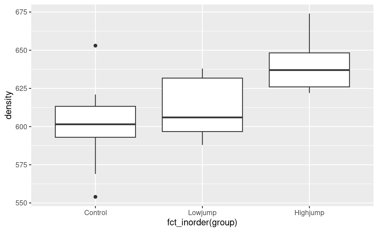

The boxplot shows that the bone density is much higher on average for the high-jumping rats than for the others; there seems to be not much difference between the control rats and the ones doing low jumping.

An annoying detail is that ggplot will put the groups in alphabetical (= nonsensical) order unless you stop it from doing so. In the data read in from the file, the jumping groups are in a sensible order, so I can use fct_inorder from forcats to arrange the group categories in the order they appear in the data.

Under the standard assumptions for analysis of variance (which we don’t assess in this post), the ANOVA \(F\)-test is obtained this way:

rats.1 <- aov(density ~ group, data = rats)
summary(rats.1)

            Df Sum Sq Mean Sq F value Pr(>F)   
group        2   7434    3717   7.978 0.0019 **
Residuals   27  12579     466                  
---
Signif. codes:  0 '***' 0.001 '**' 0.01 '*' 0.05 '.' 0.1 ' ' 1

The null hypothesis, which says that all three groups have the same mean bone density, is rejected. So, not all the groups have the same mean. But that’s all we learn here. We learn nothing about which groups differ from which, which is what we really want to know.

Some math

Let’s see how far we can get with math. Let’s assume the null hypothesis is true (that all of our \(k\) groups have the same mean \(\mu\)), and we’ll also assume that all the observations have a normal distribution with the same variance \(\sigma^2\) (a standard assumption of ANOVA), and, to make life easier, that all the groups have the same number of observations \(n\).

Let \(Y_{ij}\) denote the \(j\)th observation in group \(i\). Then, each \(Y_{ij}\) under our assumptions has independently a normal distribution with mean \(\mu\) and variance \(\sigma^2\). Hence, each group’s sample mean \(\bar{Y}_{i}\) has a normal sampling distribution with mean \(\mu\) and variance \(\sigma^2 / n\). (Having each group be the same size makes these variances the same.)

Tukey’s idea was: one of the sample means will be largest, just by chance, and one of them will be smallest, just by chance. What is the distribution of the largest one minus the smallest one? This leans on a known result: if \(X_1, \ldots X_k\) are independently normal with the same distribution, the distribution of the largest one minus the smallest one, scaled by an estimate of spread, has what is called a studentized range distribution, for which (as we used to say in the old days) tables are available: \((X_{max} - X_{min})/s\) has a studentized range distribution, which depends on \(k\) and the degrees of freedom in \(s\).

Now, since the \(\bar{Y}_{i}\) are also normal, it follows that \[(\bar{Y}_{max} -\bar{Y}_{min}) / (s / \sqrt{n})\] also has a studentized range distribution, where \(s\) in this case is the square root of a pooled estimate of variance, which is just the average of the within-group variances (because the sample size within each group is the same). To make this work, Tukey said that if you take the upper 5% point of this distribution, and scale it properly, you can say that any group means will rarely differ by this much if the null hypothesis is true, and thus that any two group means that do differ by more than this are significantly different.

The value of doing this is that you are only doing one test, based on how far apart the largest and smallest sample means might be, and applying that to all pairs of groups, so that you avoid the multiple testing problem of doing all possible two-sample \(t\)-tests.

So, say we have three groups with 10 observations in each (as in our jumping rats data). The upper 5% point of the appropriate Studentized range distribution is

q <- qtukey(0.95, nmeans = 3, df = 27)
q

[1] 3.506426

then we multiply that by the square root of the error mean square divided by its df, with an extra factor of 2 that I am not sure about:

w <- q * sqrt(466/27*2)
w

[1] 20.60112

and we say that any sample means differing by more than that are significantly different:

rats %>% 
  group_by(group) %>% 
  summarize(mean_density = mean(density))

# A tibble: 3 × 2
  group    mean_density
  <chr>           <dbl>
1 Control          601.
2 Highjump         639.
3 Lowjump          612.

Control and Lowjump are not far enough apart to be significantly different, but the two comparisons with Highjump are both significant.

In practice, we would use TukeyHSD which does all of that for us:

TukeyHSD(rats.1)

  Tukey multiple comparisons of means
    95% family-wise confidence level

Fit: aov(formula = density ~ group, data = rats)

$group
                  diff       lwr       upr     p adj
Highjump-Control  37.6  13.66604 61.533957 0.0016388
Lowjump-Control   11.4 -12.53396 35.333957 0.4744032
Lowjump-Highjump -26.2 -50.13396 -2.266043 0.0297843

with the same results.

Some simulation

Can we simulate the distribution of the difference between the highest and lowest sample means of our three groups? We have to set this up so that the null hypothesis is true, so that all three simulations come from groups with the same mean. It doesn’t matter what mean we use, but we may as well use the overall mean of our data:

rats %>% 
  summarize(grand_mean = mean(density)) %>% as.numeric() -> grand_mean
grand_mean

[1] 617.4333

gp_sd <- sqrt(466)
gp_sd

[1] 21.58703

so we simulate three groups of 10 observations from a normal distribution with mean 617.4333 and SD 21.5870, and then compare the highest mean with the lowest one. I’m putting this into a function because I’m going to build a simulation around it. The steps are:

• set up for as many samples as I want
• work rowwise
• draw a random sample of the right size with the right mean and SD in each row
• work out the mean of each sample
• stop working rowwise
• find the largest and smallest of the simulated sample means, and the difference between them
• return that difference as a number:

ksample <- function(nobs, nsample, mu, sigma) {
  tibble(sample = 1:nsample) %>% 
    rowwise() %>% 
    mutate(my_sample = list(rnorm(nobs, mu, sigma))) %>% 
    mutate(my_mean = mean(my_sample)) %>% 
    ungroup() %>% 
    summarize(mn = min(my_mean), mx = max(my_mean)) %>% 
    mutate(rnge = mx - mn) %>% 
    pull(rnge)
}

Does it work?

ksample(10, 3, grand_mean, gp_sd)

[1] 15.23404

Well, I guess that looks all right. So now let’s do this many times:

set.seed(457299)

tibble(sim = 1:1000) %>% 
  rowwise() %>% 
  mutate(rnge = ksample(10, 3, grand_mean, gp_sd)) -> ranges
ranges

# A tibble: 1,000 × 2
# Rowwise: 
     sim  rnge
   <int> <dbl>
 1     1  7.73
 2     2 25.1 
 3     3  3.45
 4     4 13.2 
 5     5 17.5 
 6     6 22.9 
 7     7 12.6 
 8     8 12.9 
 9     9 12.0 
10    10  2.92
# ℹ 990 more rows

The differences between the highest sample mean and the lowest one seem all over the place, but so it is:

ggplot(ranges, aes(x = rnge)) + geom_histogram(bins = 10)

Skewed to the right, with a lower limit of zero.

So now, let’s compare this null distribution with our actual data:

rats %>% 
  group_by(group) %>% 
  summarize(mean_density = mean(density))

# A tibble: 3 × 2
  group    mean_density
  <chr>           <dbl>
1 Control          601.
2 Highjump         639.
3 Lowjump          612.

We can get a Tukey-style P-value by taking each difference in means, and seeing how many of our simulated max mean minus min mean exceed that:

• control vs highjump, difference is 37.6:

ranges %>% count(rnge >= 37.6)

# A tibble: 1 × 2
# Rowwise: 
  `rnge >= 37.6`     n
  <lgl>          <int>
1 FALSE           1000

• control vs lowjump, difference is 11.4:

ranges %>% count(rnge >= 11.4)

# A tibble: 2 × 2
# Rowwise: 
  `rnge >= 11.4`     n
  <lgl>          <int>
1 FALSE            544
2 TRUE             456

highjump vs lowjump, difference is 26.2:

ranges %>% count(rnge >= 26.2)

# A tibble: 2 × 2
# Rowwise: 
  `rnge >= 26.2`     n
  <lgl>          <int>
1 FALSE            985
2 TRUE              15

With P-values

TukeyHSD(rats.1)

  Tukey multiple comparisons of means
    95% family-wise confidence level

Fit: aov(formula = density ~ group, data = rats)

$group
                  diff       lwr       upr     p adj
Highjump-Control  37.6  13.66604 61.533957 0.0016388
Lowjump-Control   11.4 -12.53396 35.333957 0.4744032
Lowjump-Highjump -26.2 -50.13396 -2.266043 0.0297843

Our simulated P-values were respectively 0, 0.456, and 0.015, which are very much consistent with the actual ones from Tukey’s procedure.

If you wanted to do this the way we used to do it, rather than getting P-values, you get a critical value as the 95th percentile of the simulated mean differences:

ranges %>% 
  ungroup() %>% 
  summarize(q = quantile(rnge, 0.95))

# A tibble: 1 × 1
      q
  <dbl>
1  22.5

and then you’d say that any means that differed by more than 22.5 were significantly different (the two comparisons involving Highjump) and any differing by less than that were not (Lowjump vs Control).