Chapter 28 Logistic regression with nominal response

library(nnet)
library(tidyverse)

28.1 Finding non-missing values

* This is to prepare you for something in the next question. It’s meant to be easy.

In R, the code NA stands for “missing value” or “value not known”. In R, NA should not have quotes around it. (It is a special code, not a piece of text.)

Create a vector v that contains some numbers and some missing values, using c(). Put those values into a one-column data frame.
Obtain a new column containing is.na(v). When is this true and when is this false?
The symbol ! means “not” in R (and other programming languages). What does !is.na(v) do? Create a new column containing that.
Use filter to display just the rows of your data frame that have a non-missing value of v.

28.2 European Social Survey and voting

The European Social Survey is a giant survey carried out across Europe covering demographic information, attitudes to and amount of education, politics and so on. In this question, we will investigate what might make British people vote for a certain political party.

The information for this question is in a (large) spreadsheet at link. There is also a “codebook” at link that tells you what all the variables are. The ones we will use are the last five columns of the spreadsheet, described on pages 11 onwards of the codebook. (I could have given you more, but I didn’t want to make this any more complicated than it already was.)

Read in the .csv file, and verify that you have lots of rows and columns.
* Use the codebook to find out what the columns prtvtgb, gndr, agea, eduyrs and inwtm are. What do the values 1 and 2 for gndr mean? (You don’t, at this point, have to worry about the values for the other variables.)
The three major political parties in Britain are the Conservative, Labour and Liberal Democrat. (These, for your information, correspond roughly to the Canadian Progressive Conservative, NDP and Liberal parties.) For the variable that corresponds to “political party voted for at the last election”, which values correspond to these three parties?
Normally, I would give you a tidied-up data set. But I figure you could use some practice tidying this one up. As the codebook shows, there are some numerical codes for missing values, and we want to omit those. We want just the columns prtvtgb through inwtm from the right side of the spreadsheet. Use dplyr or tidyr tools to (i) select only these columns, (ii) include the rows that correspond to people who voted for one of the three major parties, (iii) include the rows that have an age at interview less than 999, (iv) include the rows that have less than 40 years of education, (v) include the rows that are not missing on inwtm (use the idea from Question~here for (v)). The last four of those (the inclusion of rows) can be done in one go.
Why is my response variable nominal rather than ordinal? How can I tell? Which R function should I use, therefore, to fit my model?
* Take the political party voted for, and turn it into a factor, by feeding it into factor. Fit an appropriate model to predict political party voted for at the last election (as a factor) from all the other variables. Gender is really a categorical variable too, but since there are only two possible values it can be treated as a number.
We have a lot of explanatory variables. The standard way to test whether we need all of them is to take one of them out at a time, and test which ones we can remove. This is a lot of work. We won’t do that. Instead, the R function step does what you want. You feed step two things: a fitted model object, and the option trace=0 (otherwise you get a lot of output). The final part of the output from step tells you which explanatory variables you need to keep. Run step on your fitted model. Which explanatory variables need to stay in the model here?
Fit the model indicated by step (in the last part).
I didn’t think that interview length could possibly be relevant to which party a person voted for. Test whether interview length can be removed from your model of the last part. What do you conclude? (Note that step and this test may disagree.)
Use your best model to obtain predictions from some suitably chosen combinations of values of the explanatory variables that remain. (If you have quantitative explanatory variables left, you could use their first and third quartiles as values to predict from. Running summary on the data frame will get summaries of all the variables.)
What is the effect of increasing age? What is the effect of an increase in years of education?

28.3 Alligator food

What do alligators most like to eat? 219 alligators were captured in four Florida lakes. Each alligator’s stomach contents were observed, and the food that the alligator had eaten was classified into one of five categories: fish, invertebrates (such as snails or insects), reptiles (such as turtles), birds, and “other” (such as amphibians, plants or rocks). The researcher noted for each alligator what that alligator had most of in its stomach, as well as the gender of each alligator and whether it was “large” or “small” (greater or less than 2.3 metres in length). The data can be found in link. The numbers in the data set (apart from the first column) are all frequencies. (You can ignore that first column “profile”.)

Our aim is to predict food type from the other variables.

Read in the data and display the first few lines. Describe how the data are not “tidy”.
Use pivot_longer to arrange the data suitably for analysis (which will be using multinom). Demonstrate (by looking at the first few rows of your new data frame) that you now have something tidy.
What is different about this problem, compared to Question here, that would make multinom the right tool to use?
Fit a suitable multinomial model predicting food type from gender, size and lake. Does each row represent one alligator or more than one? If more than one, account for this in your modelling.
Do a test to see whether Gender should stay in the model. (This will entail fitting another model.) What do you conclude?
Predict the probability that an alligator prefers each food type, given its size, gender (if necessary) and the lake it was found in, using the more appropriate of the two models that you have fitted so far. This means (i) making a data frame for prediction, and (ii) obtaining and displaying the predicted probabilities in a way that is easy to read.
What do you think is the most important way in which the lakes differ? (Hint: look at where the biggest predicted probabilities are.)
How would you describe the major difference between the diets of the small and large alligators?

28.4 Crimes in San Francisco

The data in link is a subset of a huge dataset of crimes committed in San Francisco between 2003 and 2015. The variables are:

Dates: the date and time of the crime
Category: the category of crime, eg. “larceny” or “vandalism” (response).
Descript: detailed description of crime.
DayOfWeek: the day of the week of the crime.
PdDistrict: the name of the San Francisco Police Department district in which the crime took place.
Resolution: how the crime was resolved
Address: approximate street address of crime
X: longitude
Y: latitude

Our aim is to see whether the category of crime depends on the day of the week and the district in which it occurred. However, there are a lot of crime categories, so we will focus on the top four “interesting” ones, which are the ones included in this data file.

Some of the model-fitting takes a while (you’ll see why below). If you’re using R Markdown, you can wait for the models to fit each time you re-run your document, or insert cache=T in the top line of your code chunk (the one with r in curly brackets in it, above the actual code). Put a comma and the cache=T inside the curly brackets. What that does is to re-run that code chunk only if it changes; if it hasn’t changed it will use the saved results from last time it was run. That can save you a lot of waiting around.

Read in the data and display the dataset (or, at least, part of it).
Fit a multinomial logistic regression that predicts crime category from day of week and district. (You don’t need to look at it.) The model-fitting produces some output. (If you’re using R Markdown, that will come with it.)
Fit a model that predicts Category from only the district. Hand in the output from the fitting process as well.
Use anova to compare the two models you just obtained. What does the anova tell you?
Using your preferred model, obtain predicted probabilities that a crime will be of each of these four categories for each day of the week in the TENDERLOIN district (the name is ALL CAPS). This will mean constructing a data frame to predict from, obtaining the predictions and then displaying them suitably.
Describe briefly how the weekend days Saturday and Sunday differ from the rest.

28.5 Crimes in San Francisco – the data

The data in link is a huge dataset of crimes committed in San Francisco between 2003 and 2015. The variables are:

Dates: the date and time of the crime
Category: the category of crime, eg. “larceny” or “vandalism” (response).
Descript: detailed description of crime.
DayOfWeek: the day of the week of the crime.
PdDistrict: the name of the San Francisco Police Department district in which the crime took place.
Resolution: how the crime was resolved
Address: approximate street address of crime
X: longitude
Y: latitude

Read in the data and verify that you have these columns and a lot of rows. (The data may take a moment to read in. You will see why.)
How is the response variable here different to the one in the question about steak preferences (and therefore why would multinom from package nnet be the method of choice)?
Find out which crime categories there are, and arrange them in order of how many crimes there were in each category.
Which are the four most frequent “interesting” crime categories, that is to say, not including “other offenses” and “non-criminal”? Get them into a vector called my.crimes. See if you can find a way of doing this that doesn’t involve typing them in (for full marks).
(Digression, but needed for the next part.) The R vector letters contains the lowercase letters from a to z. Consider the vector ('a','m',3,'Q'). Some of these are found amongst the lowercase letters, and some not. Type these into a vector v and explain briefly why v %in% letters produces what it does.
We are going to filter only the rows of our data frame that have one of the crimes in my.crimes as their Category. Also, select only the columns Category, DayOfWeek and PdDistrict. Save the resulting data frame and display its structure. (You should have a lot fewer rows than you did before.)
Save these data in a file sfcrime1.csv.

28.6 What sports do these athletes play?

The data at link are physical and physiological measurements of 202 male and female Australian elite athletes. The data values are separated by tabs. We are going to see whether we can predict the sport an athlete plays from their height and weight.

The sports, if you care, are respectively basketball, “field athletics” (eg. shot put, javelin throw, long jump etc.), gymnastics, netball, rowing, swimming, 400m running, tennis, sprinting (100m or 200m running), water polo.

Read in the data and display the first few rows.
Make a scatterplot of height vs. weight, with the points coloured by what sport the athlete plays. Put height on the \(x\)-axis and weight on the \(y\)-axis.
Explain briefly why a multinomial model (multinom from nnet) would be the best thing to use to predict sport played from the other variables.
Fit a suitable model for predicting sport played from height and weight. (You don’t need to look at the results.) 100 steps isn’t quite enough, so set maxit equal to a larger number to allow the estimation to finish.
Demonstrate using anova that Wt should not be removed from this model.
Make a data frame consisting of all combinations of Ht 160, 180 and 200 (cm), and Wt 50, 75, and 100 (kg), and use it to obtain predicted probabilities of athletes of those heights and weights playing each of the sports. Display the results. You might have to display them smaller, or reduce the number of decimal places³⁶ to fit them on the page.
For an athlete who is 180 cm tall and weighs 100 kg, what sport would you guess they play? How sure are you that you are right? Explain briefly.

My solutions follow:

28.7 Finding non-missing values

* This is to prepare you for something in the next question. It’s meant to be easy.

In R, the code NA stands for “missing value” or “value not known”. In R, NA should not have quotes around it. (It is a special code, not a piece of text.)

Create a vector v that contains some numbers and some missing values, using c(). Put those values into a one-column data frame.

Solution

Like this. The arrangement of numbers and missing values doesn’t matter, as long as you have some of each:

v <- c(1, 2, NA, 4, 5, 6, 9, NA, 11)
mydata <- tibble(v)
mydata

## # A tibble: 9 × 1
##       v
##   <dbl>
## 1     1
## 2     2
## 3    NA
## 4     4
## 5     5
## 6     6
## 7     9
## 8    NA
## 9    11

This has one column called v.

\(\blacksquare\)

Obtain a new column containing is.na(v). When is this true and when is this false?

Solution

mydata <- mydata %>% mutate(isna = is.na(v))
mydata

## # A tibble: 9 × 2
##       v isna 
##   <dbl> <lgl>
## 1     1 FALSE
## 2     2 FALSE
## 3    NA TRUE 
## 4     4 FALSE
## 5     5 FALSE
## 6     6 FALSE
## 7     9 FALSE
## 8    NA TRUE 
## 9    11 FALSE

This is TRUE if the corresponding element of v is missing (in my case, the third value and the second-last one), and FALSE otherwise (when there is an actual value there).

\(\blacksquare\)

The symbol ! means “not” in R (and other programming languages). What does !is.na(v) do? Create a new column containing that.

Solution

Try it and see. Give it whatever name you like. My name reflects that I know what it’s going to do:

mydata <- mydata %>% mutate(notisna = !is.na(v))
mydata

## # A tibble: 9 × 3
##       v isna  notisna
##   <dbl> <lgl> <lgl>  
## 1     1 FALSE TRUE   
## 2     2 FALSE TRUE   
## 3    NA TRUE  FALSE  
## 4     4 FALSE TRUE   
## 5     5 FALSE TRUE   
## 6     6 FALSE TRUE   
## 7     9 FALSE TRUE   
## 8    NA TRUE  FALSE  
## 9    11 FALSE TRUE

This is the logical opposite of is.na: it’s true if there is a value, and false if it’s missing.

\(\blacksquare\)

Use filter to display just the rows of your data frame that have a non-missing value of v.

Solution

filter takes a column to say which rows to pick, in which case the column should contain something that either is TRUE or FALSE, or something that can be interpreted that way:

mydata %>% filter(notisna)

## # A tibble: 7 × 3
##       v isna  notisna
##   <dbl> <lgl> <lgl>  
## 1     1 FALSE TRUE   
## 2     2 FALSE TRUE   
## 3     4 FALSE TRUE   
## 4     5 FALSE TRUE   
## 5     6 FALSE TRUE   
## 6     9 FALSE TRUE   
## 7    11 FALSE TRUE

or you can provide filter something that can be calculated from what’s in the data frame, and also returns something that is either true or false:

mydata %>% filter(!is.na(v))

## # A tibble: 7 × 3
##       v isna  notisna
##   <dbl> <lgl> <lgl>  
## 1     1 FALSE TRUE   
## 2     2 FALSE TRUE   
## 3     4 FALSE TRUE   
## 4     5 FALSE TRUE   
## 5     6 FALSE TRUE   
## 6     9 FALSE TRUE   
## 7    11 FALSE TRUE

In either case, I only have non-missing values of v.

\(\blacksquare\)

28.8 European Social Survey and voting

Read in the .csv file, and verify that you have lots of rows and columns.

Solution

The obvious way. Printing it out will display some of the data and tell you how many rows and columns you have:

my_url <- "http://ritsokiguess.site/datafiles/ess.csv"
ess <- read_csv(my_url)

## Rows: 2286 Columns: 17
## ── Column specification ────────────────────────────────────────────────────────
## Delimiter: ","
## chr  (4): cntry, cname, cproddat, name
## dbl (13): cedition, cseqno, essround, edition, idno, dweight, pspwght, pweig...
## 
## ℹ Use `spec()` to retrieve the full column specification for this data.
## ℹ Specify the column types or set `show_col_types = FALSE` to quiet this message.

ess

## # A tibble: 2,286 × 17
##    cntry cname    cedition cproddat cseqno name  essround edition   idno dweight
##    <chr> <chr>       <dbl> <chr>     <dbl> <chr>    <dbl>   <dbl>  <dbl>   <dbl>
##  1 GB    ESS1-6e…        1 26.11.2… 134168 ESS6…        6     2.1 101014   1.01 
##  2 GB    ESS1-6e…        1 26.11.2… 134169 ESS6…        6     2.1 101048   2.02 
##  3 GB    ESS1-6e…        1 26.11.2… 134170 ESS6…        6     2.1 101055   1.01 
##  4 GB    ESS1-6e…        1 26.11.2… 134171 ESS6…        6     2.1 101089   0.505
##  5 GB    ESS1-6e…        1 26.11.2… 134172 ESS6…        6     2.1 101097   0.505
##  6 GB    ESS1-6e…        1 26.11.2… 134173 ESS6…        6     2.1 101113   1.01 
##  7 GB    ESS1-6e…        1 26.11.2… 134174 ESS6…        6     2.1 101121   0.505
##  8 GB    ESS1-6e…        1 26.11.2… 134175 ESS6…        6     2.1 101139   0.505
##  9 GB    ESS1-6e…        1 26.11.2… 134176 ESS6…        6     2.1 101154   1.01 
## 10 GB    ESS1-6e…        1 26.11.2… 134177 ESS6…        6     2.1 101170   1.01 
## # … with 2,276 more rows, and 7 more variables: pspwght <dbl>, pweight <dbl>,
## #   prtvtgb <dbl>, gndr <dbl>, agea <dbl>, eduyrs <dbl>, inwtm <dbl>

2286 rows and 17 columns.

\(\blacksquare\)

* Use the codebook to find out what the columns prtvtgb, gndr, agea, eduyrs and inwtm are. What do the values 1 and 2 for gndr mean? (You don’t, at this point, have to worry about the values for the other variables.)

Solution

Respectively, political party voted for at last election, gender (of respondent), age at interview, years of full-time education, length of interview (in minutes). For gndr, male is 1 and female is 2.

\(\blacksquare\)

The three major political parties in Britain are the Conservative, Labour and Liberal Democrat. (These, for your information, correspond roughly to the Canadian Progressive Conservative, NDP and Liberal parties.) For the variable that corresponds to “political party voted for at the last election”, which values correspond to these three parties?

Solution

1, 2 and 3 respectively. (That was easy!)

\(\blacksquare\)

Normally, I would give you a tidied-up data set. But I figure you could use some practice tidying this one up. As the codebook shows, there are some numerical codes for missing values, and we want to omit those. We want just the columns prtvtgb through inwtm from the right side of the spreadsheet. Use dplyr or tidyr tools to (i) select only these columns, (ii) include the rows that correspond to people who voted for one of the three major parties, (iii) include the rows that have an age at interview less than 999, (iv) include the rows that have less than 40 years of education, (v) include the rows that are not missing on inwtm (use the idea from Question~here for (v)). The last four of those (the inclusion of rows) can be done in one go.

Solution

The major parties are numbered 1, 2 and 3, so we can select the ones less than 4 (or <=3). The reference back to the last question is a hint to use !is.na(). It also works to use drop_na, if you are familiar with that.

ess %>%
  select(prtvtgb:inwtm) %>%
  filter(prtvtgb < 4, agea < 999, eduyrs < 40, !is.na(inwtm)) -> ess.major

You might get a weird error in select, something about “unused argument”. If this happens to you, it’s not because you used select wrong, it’s because you used the wrong select! There is one in MASS, and you need to make sure that this package is “detached” so that you use the select you want, namely the one in dplyr, loaded with the tidyverse. Use the instructions at the end of the mobile phones question or the abortion question to do this.

The other way around this is to say, instead of select, dplyr::select with two colons. This means “the select that lives in dplyr, no other”, and is what Wikipedia calls “disambiguation”: out of several things with the same name, you say which one you mean.

If you do the pipeline, you will probably not get it right the first time. (I didn’t.) For debugging, try out one step at a time, and summarize what you have so far, so that you can check it for correctness. A handy trick for that is to make the last piece of your pipeline summary(), which produces a summary of the columns of the resulting data frame. For example, I first did this (note that my filter is a lot simpler than the one above):

ess %>%
  select(prtvtgb:inwtm) %>%
  filter(prtvtgb < 4, !is.na(inwtm)) %>%
  summary()

##     prtvtgb           gndr            agea            eduyrs     
##  Min.   :1.000   Min.   :1.000   Min.   : 18.00   Min.   : 0.00  
##  1st Qu.:1.000   1st Qu.:1.000   1st Qu.: 44.00   1st Qu.:11.00  
##  Median :2.000   Median :2.000   Median : 58.00   Median :13.00  
##  Mean   :1.803   Mean   :1.572   Mean   : 61.74   Mean   :14.23  
##  3rd Qu.:2.000   3rd Qu.:2.000   3rd Qu.: 71.00   3rd Qu.:16.00  
##  Max.   :3.000   Max.   :2.000   Max.   :999.00   Max.   :88.00  
##      inwtm       
##  Min.   :  7.00  
##  1st Qu.: 35.00  
##  Median : 41.00  
##  Mean   : 43.54  
##  3rd Qu.: 50.00  
##  Max.   :160.00

The mean of a categorical variable like party voted for or gender doesn’t make much sense, but it looks as if all the values are sensible ones (1 to 3 and 1, 2 respectively). However, the maximum values of age and years of education look like missing value codes, hence the other requirements I put in the question.³⁷

Displaying as the last step of your pipeline also works, but the advantage of summary is that you get to see whether there are any unusual values, in this case unusually large values that are missing value codes.

\(\blacksquare\)

Why is my response variable nominal rather than ordinal? How can I tell? Which R function should I use, therefore, to fit my model?

Solution

The response variable is political party voted for. There is no (obvious) ordering to this (unless you want to try to place the parties on a left-right spectrum), so this is nominal, and you’ll need multinom from package nnet.

If I had included the minor parties and you were working on a left-right spectrum, you would have had to decide where to put the somewhat libertarian Greens³⁸ or the parties that exist only in Northern Ireland.³⁹

\(\blacksquare\)

* Take the political party voted for, and turn it into a factor, by feeding it into factor. Fit an appropriate model to predict political party voted for at the last election (as a factor) from all the other variables. Gender is really a categorical variable too, but since there are only two possible values it can be treated as a number.

Solution

This, or something like it. multinom lives in package nnet, which you’ll have to install first if you haven’t already:

library(nnet)
ess.1 <- multinom(factor(prtvtgb) ~ gndr + agea + eduyrs + inwtm, data = ess.major)

## # weights:  18 (10 variable)
## initial  value 1343.602829 
## iter  10 value 1256.123798
## final  value 1247.110080 
## converged

Or create a factor version of your response in the data frame first:

ess.major <- ess.major %>% mutate(party = factor(prtvtgb))

and then:

ess.1a <- multinom(party ~ gndr + agea + eduyrs + inwtm, data = ess.major)

## # weights:  18 (10 variable)
## initial  value 1343.602829 
## iter  10 value 1256.123798
## final  value 1247.110080 
## converged

\(\blacksquare\)

We have a lot of explanatory variables. The standard way to test whether we need all of them is to take one of them out at a time, and test which ones we can remove. This is a lot of work. We won’t do that. Instead, the R function step does what you want. You feed step two things: a fitted model object, and the option trace=0 (otherwise you get a lot of output). The final part of the output from step tells you which explanatory variables you need to keep. Run step on your fitted model. Which explanatory variables need to stay in the model here?

Solution

I tried to give you lots of hints here:

ess.2a <- step(ess.1, trace = 0)

## trying - gndr 
## trying - agea 
## trying - eduyrs 
## trying - inwtm 
## # weights:  15 (8 variable)
## initial  value 1343.602829 
## iter  10 value 1248.343563
## final  value 1248.253638 
## converged
## trying - agea 
## trying - eduyrs 
## trying - inwtm

ess.2a

## Call:
## multinom(formula = factor(prtvtgb) ~ agea + eduyrs + inwtm, data = ess.major)
## 
## Coefficients:
##   (Intercept)        agea     eduyrs       inwtm
## 2    1.632266 -0.02153694 -0.0593757 0.009615167
## 3   -1.281031 -0.01869263  0.0886487 0.009337084
## 
## Residual Deviance: 2496.507 
## AIC: 2512.507

If you didn’t save your output in a variable, you’ll get my last bit automatically.

The end of the output gives us coefficients for (and thus tells us we need to keep) age, years of education and interview length.

The actual numbers don’t mean much; it’s the indication that the variable has stayed in the model that makes a difference.⁴⁰

If you’re wondering about the process: first step tries to take out each explanatory variable, one at a time, from the starting model (the one that contains all the variables). Then it finds the best model out of those and fits it. (It doesn’t tell us which model this is, but evidently it’s the one without gender.) Then it takes that model and tries to remove its explanatory variables one at a time (there are only three of them left). Having decided it cannot remove any of them, it stops, and shows us what’s left.

Leaving out the trace=0 shows more output and more detail on the process, but I figured this was enough (and this way, you don’t have to wade through all of that output). Try values like 1 or 2 for trace and see what you get.

\(\blacksquare\)

Fit the model indicated by step (in the last part).

Solution

Copy and paste, and take out the variables you don’t need. Or, better, save the output from step in a variable. This then becomes a fitted model object and you can look at it any of the ways you can look at a model fit. I found that gender needed to be removed, but if yours is different, follow through with whatever your step said to do.

ess.2 <- multinom(party ~ agea + eduyrs + inwtm, data = ess.major)

## # weights:  15 (8 variable)
## initial  value 1343.602829 
## iter  10 value 1248.343563
## final  value 1248.253638 
## converged

If you saved the output from step, you’ll already have this and you don’t need to do it again:

anova(ess.2, ess.2a)

## Likelihood ratio tests of Multinomial Models
## 
## Response: party
## Response: factor(prtvtgb)
##                   Model Resid. df Resid. Dev   Test    Df LR stat. Pr(Chi)
## 1 agea + eduyrs + inwtm      2438   2496.507                              
## 2 agea + eduyrs + inwtm      2438   2496.507 1 vs 2     0        0       1

Same model.

\(\blacksquare\)

I didn’t think that interview length could possibly be relevant to which party a person voted for. Test whether interview length can be removed from your model of the last part. What do you conclude? (Note that step and this test may disagree.)

Solution

Fit the model without inwtm:

ess.3 <- multinom(party ~ agea + eduyrs, data = ess.major)

## # weights:  12 (6 variable)
## initial  value 1343.602829 
## iter  10 value 1250.418281
## final  value 1250.417597 
## converged

and then use anova to compare them:

anova(ess.3, ess.2)

## Likelihood ratio tests of Multinomial Models
## 
## Response: party
##                   Model Resid. df Resid. Dev   Test    Df LR stat.   Pr(Chi)
## 1         agea + eduyrs      2440   2500.835                                
## 2 agea + eduyrs + inwtm      2438   2496.507 1 vs 2     2 4.327917 0.1148695

The P-value, 0.1149, is not small, which says that the smaller model is good, ie. the one without interview length.

I thought drop1 would also work here, but it appears not to:

drop1(ess.1, test = "Chisq")

## trying - gndr

## Error in if (trace) {: argument is not interpretable as logical

I think that’s a bug in multinom, since normally if step works, then drop1 will work too (normally step uses drop1).

The reason for the disagreement between step and anova is that step will tend to keep marginal explanatory variables, that is, ones that are “potentially interesting” but whose P-values might not be less than 0.05. There is still no substitute for your judgement in figuring out what to do! step uses a thing called AIC to decide what to do, rather than actually doing a test. If you know about “adjusted R-squared” in choosing explanatory variables for a regression, it’s the same idea: a variable can be not quite significant but still make the adjusted R-squared go up (typically only a little).

\(\blacksquare\)

Use your best model to obtain predictions from some suitably chosen combinations of values of the explanatory variables that remain. (If you have quantitative explanatory variables left, you could use their first and third quartiles as values to predict from. Running summary on the data frame will get summaries of all the variables.)

Solution

First make our new data frame of values to predict from. crossing is our friend. You can use quantile or summary to find the quartiles. I only had agea and eduyrs left, having decided that interview time really ought to come out:

summary(ess.major)

##     prtvtgb           gndr            agea           eduyrs     
##  Min.   :1.000   Min.   :1.000   Min.   :18.00   Min.   : 0.00  
##  1st Qu.:1.000   1st Qu.:1.000   1st Qu.:44.00   1st Qu.:11.00  
##  Median :2.000   Median :2.000   Median :58.00   Median :13.00  
##  Mean   :1.803   Mean   :1.574   Mean   :57.19   Mean   :13.45  
##  3rd Qu.:2.000   3rd Qu.:2.000   3rd Qu.:71.00   3rd Qu.:16.00  
##  Max.   :3.000   Max.   :2.000   Max.   :94.00   Max.   :33.00  
##      inwtm       party  
##  Min.   :  7.0   1:484  
##  1st Qu.: 35.0   2:496  
##  Median : 41.0   3:243  
##  Mean   : 43.7          
##  3rd Qu.: 50.0          
##  Max.   :160.0

Quartiles for age are 44 and 71, and for years of education are 11 and 16.

This time, instead of predicting for variable values that predictions chooses for us (like a five-number summary), we are predicting for “custom” values, ones that we chose. To set that up, the marginaleffects way is to use datagrid like this:

new <- datagrid(model = ess.3, agea = c(44, 71), eduyrs = c(11, 16))
new

##    agea eduyrs
## 1:   44     11
## 2:   44     16
## 3:   71     11
## 4:   71     16

What datagrid does is to make all combinations of your variable values, and along with that, to use “typical” values for the others: the mean, in the case of quantitative variables like inwtm, and the most common category for categorical ones like party. If you feed datagrid a model first, it only includes variables in that model, which is easier to make sense of:

datagrid(newdata = ess.major, agea = c(44, 71), eduyrs = c(11, 16))

##     prtvtgb     gndr    inwtm party agea eduyrs
## 1: 1.802944 1.573998 43.69665     2   44     11
## 2: 1.802944 1.573998 43.69665     2   44     16
## 3: 1.802944 1.573998 43.69665     2   71     11
## 4: 1.802944 1.573998 43.69665     2   71     16

The other variables don’t make much sense, since they are really categorical but expressed as numbers, but they are not in the best model, so that doesn’t do any harm. (In other cases, you might need to be more careful.)

Next, we feed this into predictions, using the above dataframe as newdata, and with our best model, ess.3 (the one without interview length). The results might confuse you at first, since you will probably get an error:

predictions(ess.3, newdata = new)

## Error: The `type` argument for models of class `multinom` must be an element of: probs

The error message gives you a hint about what to do: add a type = "probs" to predictions (which is a consequence of how multinom works):

predictions(ess.3, newdata = new, type = "probs")

##    rowid  type group predicted    std.error agea eduyrs
## 1      1 probs     1 0.3331882 1.174676e-01   44     11
## 2      2 probs     1 0.3471967 1.137748e-01   44     16
## 3      3 probs     1 0.4551429 7.897207e-02   71     11
## 4      4 probs     1 0.4675901 7.370938e-02   71     16
## 5      1 probs     2 0.5093898 1.174676e-01   44     11
## 6      2 probs     2 0.3955666 1.137748e-01   44     16
## 7      3 probs     2 0.4085120 7.897207e-02   71     11
## 8      4 probs     2 0.3127561 7.370938e-02   71     16
## 9      1 probs     3 0.1574220 3.404357e-18   44     11
## 10     2 probs     3 0.2572367 5.450831e-18   44     16
## 11     3 probs     3 0.1363451 1.480736e-29   71     11
## 12     4 probs     3 0.2196538 2.331425e-29   71     16

There are twelve rows for our four predictions, because there are three predictions for each of our four “people”: the probabilities of each one voting for each of the three parties. The party predicted for is in the column group, and the probability of each person (labelled by rowid) voting for that party is in predicted. Let’s simplify things by keeping only those columns and the ones we are predicting for:

predictions(ess.3, newdata = new, type = "probs") %>% 
  select(rowid, group, predicted, agea, eduyrs)

##    rowid group predicted agea eduyrs
## 1      1     1 0.3331882   44     11
## 2      2     1 0.3471967   44     16
## 3      3     1 0.4551429   71     11
## 4      4     1 0.4675901   71     16
## 5      1     2 0.5093898   44     11
## 6      2     2 0.3955666   44     16
## 7      3     2 0.4085120   71     11
## 8      4     2 0.3127561   71     16
## 9      1     3 0.1574220   44     11
## 10     2     3 0.2572367   44     16
## 11     3     3 0.1363451   71     11
## 12     4     3 0.2196538   71     16

and then pivot wider to get all three predictions for each person on one line:

predictions(ess.3, newdata = new, type = "probs") %>% 
  select(rowid, group, predicted, agea, eduyrs) %>% 
  pivot_wider(names_from = group, values_from = predicted)

## # A tibble: 4 × 6
##   rowid  agea eduyrs   `1`   `2`   `3`
##   <int> <dbl>  <dbl> <dbl> <dbl> <dbl>
## 1     1    44     11 0.333 0.509 0.157
## 2     2    44     16 0.347 0.396 0.257
## 3     3    71     11 0.455 0.409 0.136
## 4     4    71     16 0.468 0.313 0.220

\(\blacksquare\)

What is the effect of increasing age? What is the effect of an increase in years of education?

Solution

To assess the effect of age, hold years of education constant. Thus, compare lines 1 and 3 (or 2 and 4): increasing age tends to increase the chance that a person will vote Conservative (party 1), and decrease the chance that a person will vote Labour (party 2). There doesn’t seem to be much effect of age on the chance that a person will vote Liberal Democrat.

To assess education, hold age constant, and thus compare rows 1 and 2 (or rows 3 and 4). This time, there isn’t much effect on the chances of voting Conservative, but as education increases, the chance of voting Labour goes down, and the chance of voting Liberal Democrat goes up.

A little history: back 150 or so years ago, Britain had two political parties, the Tories and the Whigs. The Tories became the Conservative party (and hence, in Britain and in Canada, the Conservatives are nicknamed Tories⁴¹). The Whigs became Liberals. At about the same time as working people got to vote (not women, yet, but working men) the Labour Party came into existence. The Labour Party has always been affiliated with working people and trades unions, like the NDP here. But power has typically alternated between Conservative and Labour goverments, with the Liberals as a third party. In the 1980s a new party called the Social Democrats came onto the scene, but on realizing that they couldn’t make much of a dent by themselves, they merged with the Liberals to form the Liberal Democrats, which became a slightly stronger third party.

I was curious about what the effect of interview length would be. Presumably, the effect is small, but I have no idea which way it would be. To assess this, this is predictions again, but this time we can let predictions pick some values for inwtm for us, and leave everything else at their mean. We have to remember to use the model ess.2 that contained interview length, this time:

predictions(ess.2, variables = "inwtm", type = "probs") %>% 
  select(rowid, group, predicted, agea, eduyrs, inwtm) %>% 
  pivot_wider(names_from = group, values_from = predicted)

## # A tibble: 5 × 7
##   rowid  agea eduyrs inwtm   `1`   `2`   `3`
##   <int> <dbl>  <dbl> <dbl> <dbl> <dbl> <dbl>
## 1     1  57.2   13.5     7 0.487 0.350 0.163
## 2     2  57.2   13.5    35 0.421 0.396 0.183
## 3     3  57.2   13.5    41 0.407 0.405 0.188
## 4     4  57.2   13.5    50 0.387 0.420 0.194
## 5     5  57.2   13.5   160 0.181 0.566 0.253

As interview length goes up (for a respondent with average age and years of education, though the pattern would be the same for people of different ages and different amounts of education), the respondent is less likely to vote Conservative (party 1), and more likely to vote for one of the other two parties.

But, as we suspected, the effect is small (except for that very long interview length) and not really worth worrying about.

\(\blacksquare\)

28.9 Alligator food

Our aim is to predict food type from the other variables.

Read in the data and display the first few lines. Describe how the data are not “tidy”.

Solution

Separated by exactly one space:

my_url <- "http://ritsokiguess.site/datafiles/alligator.txt"
gators.orig <- read_delim(my_url, " ")

## Rows: 16 Columns: 9
## ── Column specification ────────────────────────────────────────────────────────
## Delimiter: " "
## chr (3): Gender, Size, Lake
## dbl (6): profile, Fish, Invertebrate, Reptile, Bird, Other
## 
## ℹ Use `spec()` to retrieve the full column specification for this data.
## ℹ Specify the column types or set `show_col_types = FALSE` to quiet this message.

gators.orig

## # A tibble: 16 × 9
##    profile Gender Size  Lake      Fish Invertebrate Reptile  Bird Other
##      <dbl> <chr>  <chr> <chr>    <dbl>        <dbl>   <dbl> <dbl> <dbl>
##  1       1 f      <2.3  george       3            9       1     0     1
##  2       2 m      <2.3  george      13           10       0     2     2
##  3       3 f      >2.3  george       8            1       0     0     1
##  4       4 m      >2.3  george       9            0       0     1     2
##  5       5 f      <2.3  hancock     16            3       2     2     3
##  6       6 m      <2.3  hancock      7            1       0     0     5
##  7       7 f      >2.3  hancock      3            0       1     2     3
##  8       8 m      >2.3  hancock      4            0       0     1     2
##  9       9 f      <2.3  oklawaha     3            9       1     0     2
## 10      10 m      <2.3  oklawaha     2            2       0     0     1
## 11      11 f      >2.3  oklawaha     0            1       0     1     0
## 12      12 m      >2.3  oklawaha    13            7       6     0     0
## 13      13 f      <2.3  trafford     2            4       1     1     4
## 14      14 m      <2.3  trafford     3            7       1     0     1
## 15      15 f      >2.3  trafford     0            1       0     0     0
## 16      16 m      >2.3  trafford     8            6       6     3     5

The last five columns are all frequencies. Or, one of the variables (food type) is spread over five columns instead of being contained in one. Either is good.

My choice of “temporary” name reflects that I’m going to obtain a “tidy” data frame called gators in a moment.

\(\blacksquare\)

Use pivot_longer to arrange the data suitably for analysis (which will be using multinom). Demonstrate (by looking at the first few rows of your new data frame) that you now have something tidy.

Solution

I’m creating my “official” data frame here:

gators.orig %>% 
  pivot_longer(Fish:Other, names_to = "Food.type", values_to = "Frequency") -> gators
gators

## # A tibble: 80 × 6
##    profile Gender Size  Lake   Food.type    Frequency
##      <dbl> <chr>  <chr> <chr>  <chr>            <dbl>
##  1       1 f      <2.3  george Fish                 3
##  2       1 f      <2.3  george Invertebrate         9
##  3       1 f      <2.3  george Reptile              1
##  4       1 f      <2.3  george Bird                 0
##  5       1 f      <2.3  george Other                1
##  6       2 m      <2.3  george Fish                13
##  7       2 m      <2.3  george Invertebrate        10
##  8       2 m      <2.3  george Reptile              0
##  9       2 m      <2.3  george Bird                 2
## 10       2 m      <2.3  george Other                2
## # … with 70 more rows

I gave my column names Capital Letters to make them consistent with the others (and in an attempt to stop infesting my brain with annoying variable-name errors when I fit models later).

Looking at the first few lines reveals that I now have a column of food types and one column of frequencies, both of which are what I wanted. I can check that I have all the different food types by finding the distinct ones:

gators %>% distinct(Food.type)

## # A tibble: 5 × 1
##   Food.type   
##   <chr>       
## 1 Fish        
## 2 Invertebrate
## 3 Reptile     
## 4 Bird        
## 5 Other

(Think about why count would be confusing here.)

Note that Food.type is text (chr) rather than being a factor. I’ll hold my breath and see what happens when I fit a model where it is supposed to be a factor.

\(\blacksquare\)

What is different about this problem, compared to Question here, that would make multinom the right tool to use?

Solution

Look at the response variable Food.type (or whatever you called it): this has multiple categories, but they are not ordered in any logical way. Thus, in short, a nominal response.

\(\blacksquare\)

Fit a suitable multinomial model predicting food type from gender, size and lake. Does each row represent one alligator or more than one? If more than one, account for this in your modelling.

Solution

Each row of the tidy gators represents as many alligators as are in the Frequency column. That is, if you look at female small alligators in Lake George that ate mainly fish, there are three of those.⁴² This to remind you to include the weights piece, otherwise multinom will assume that you have one observation per line and not as many as the number in Frequency.

That is the reason that count earlier would have been confusing: it would have told you how many rows contained each food type, rather than how many alligators, and these would have been different:

gators %>% count(Food.type)

## # A tibble: 5 × 2
##   Food.type        n
##   <chr>        <int>
## 1 Bird            16
## 2 Fish            16
## 3 Invertebrate    16
## 4 Other           16
## 5 Reptile         16

gators %>% count(Food.type, wt = Frequency)

## # A tibble: 5 × 2
##   Food.type        n
##   <chr>        <dbl>
## 1 Bird            13
## 2 Fish            94
## 3 Invertebrate    61
## 4 Other           32
## 5 Reptile         19

Each food type appears on 16 rows, but is the favoured diet of very different numbers of alligators. Note the use of wt= to specify a frequency variable.⁴³

You ought to understand why those are different.

All right, back to modelling:

library(nnet)
gators.1 <- multinom(Food.type ~ Gender + Size + Lake,
  weights = Frequency, data = gators
)

## # weights:  35 (24 variable)
## initial  value 352.466903 
## iter  10 value 270.228588
## iter  20 value 268.944257
## final  value 268.932741 
## converged

This worked, even though Food.type was actually text. I guess it got converted to a factor. The ordering of the levels doesn’t matter here anyway, since this is not an ordinal model.

No need to look at it, since the output is kind of confusing anyway:

summary(gators.1)

## Call:
## multinom(formula = Food.type ~ Gender + Size + Lake, data = gators, 
##     weights = Frequency)
## 
## Coefficients:
##              (Intercept)     Genderm   Size>2.3 Lakehancock Lakeoklawaha
## Fish           2.4322304  0.60674971 -0.7308535  -0.5751295    0.5513785
## Invertebrate   2.6012531  0.14378459 -2.0671545  -2.3557377    1.4645820
## Other          1.0014505  0.35423803 -1.0214847   0.1914537    0.5775317
## Reptile       -0.9829064 -0.02053375 -0.1741207   0.5534169    3.0807416
##              Laketrafford
## Fish          -1.23681053
## Invertebrate  -0.08096493
## Other          0.32097943
## Reptile        1.82333205
## 
## Std. Errors:
##              (Intercept)   Genderm  Size>2.3 Lakehancock Lakeoklawaha
## Fish           0.7706940 0.6888904 0.6523273   0.7952147     1.210229
## Invertebrate   0.7917210 0.7292510 0.7084028   0.9463640     1.232835
## Other          0.8747773 0.7623738 0.7250455   0.9072182     1.374545
## Reptile        1.2827234 0.9088217 0.8555051   1.3797755     1.591542
##              Laketrafford
## Fish            0.8661187
## Invertebrate    0.8814625
## Other           0.9589807
## Reptile         1.3388017
## 
## Residual Deviance: 537.8655 
## AIC: 585.8655

You get one coefficient for each variable (along the top) and for each response group (down the side), using the first group as a baseline everywhere. These numbers are hard to interpret; doing predictions is much easier.

\(\blacksquare\)

Do a test to see whether Gender should stay in the model. (This will entail fitting another model.) What do you conclude?

Solution

The other model to fit is the one without the variable you’re testing:

gators.2 <- update(gators.1, . ~ . - Gender)

## # weights:  30 (20 variable)
## initial  value 352.466903 
## iter  10 value 272.246275
## iter  20 value 270.046891
## final  value 270.040139 
## converged

I did update here to show you that it works, but of course there’s no problem in just writing out the whole model again and taking out Gender, preferably by copying and pasting:

gators.2x <- multinom(Food.type ~ Size + Lake,
  weights = Frequency, data = gators
)

## # weights:  30 (20 variable)
## initial  value 352.466903 
## iter  10 value 272.246275
## iter  20 value 270.046891
## final  value 270.040139 
## converged

and then you compare the models with and without Gender using anova:

anova(gators.2, gators.1)

## Likelihood ratio tests of Multinomial Models
## 
## Response: Food.type
##                  Model Resid. df Resid. Dev   Test    Df LR stat.   Pr(Chi)
## 1          Size + Lake       300   540.0803                                
## 2 Gender + Size + Lake       296   537.8655 1 vs 2     4 2.214796 0.6963214

The P-value is not small, so the two models fit equally well, and therefore we should go with the smaller, simpler one: that is, the one without Gender.

Sometimes drop1 works here too (and sometimes it doesn’t, for reasons I haven’t figured out):

drop1(gators.1, test = "Chisq")

## trying - Gender

## Error in if (trace) {: argument is not interpretable as logical

I don’t even know what this error message means, never mind what to do about it.

\(\blacksquare\)

Predict the probability that an alligator prefers each food type, given its size, gender (if necessary) and the lake it was found in, using the more appropriate of the two models that you have fitted so far. This means (i) making a data frame for prediction, and (ii) obtaining and displaying the predicted probabilities in a way that is easy to read.

Solution

Our best model gators.2 contains size and lake, so we need to predict for all combinations of those.

You might think of this first, which is easiest:

predictions(gators.2, variables = c("Size", "Lake"), type = "probs")

##     rowid  type        group   predicted   std.error Food.type Size     Lake
## 1       1 probs         Bird 0.029671502 0.026490803      Fish <2.3   george
## 2       2 probs         Bird 0.029671502 0.026490803      Fish <2.3   george
## 3       3 probs         Bird 0.029671502 0.026490803      Fish <2.3   george
## 4       4 probs         Bird 0.029671502 0.026490803      Fish <2.3   george
## 5       5 probs         Bird 0.070400215 0.014591121      Fish <2.3  hancock
## 6       6 probs         Bird 0.070400215 0.014591121      Fish <2.3  hancock
## 7       7 probs         Bird 0.070400215 0.014591121      Fish <2.3  hancock
## 8       8 probs         Bird 0.070400215 0.014591121      Fish <2.3  hancock
## 9       9 probs         Bird 0.008818267 0.031423530      Fish <2.3 oklawaha
## 10     10 probs         Bird 0.008818267 0.031423530      Fish <2.3 oklawaha
## 11     11 probs         Bird 0.008818267 0.031423530      Fish <2.3 oklawaha
## 12     12 probs         Bird 0.008818267 0.031423530      Fish <2.3 oklawaha
## 13     13 probs         Bird 0.035892547 0.030455498      Fish <2.3 trafford
## 14     14 probs         Bird 0.035892547 0.030455498      Fish <2.3 trafford
## 15     15 probs         Bird 0.035892547 0.030455498      Fish <2.3 trafford
## 16     16 probs         Bird 0.035892547 0.030455498      Fish <2.3 trafford
## 17     17 probs         Bird 0.081071082 0.028409610      Fish >2.3   george
## 18     18 probs         Bird 0.081071082 0.028409610      Fish >2.3   george
## 19     19 probs         Bird 0.081071082 0.028409610      Fish >2.3   george
## 20     20 probs         Bird 0.081071082 0.028409610      Fish >2.3   george
## 21     21 probs         Bird 0.140898571 0.033231369      Fish >2.3  hancock
## 22     22 probs         Bird 0.140898571 0.033231369      Fish >2.3  hancock
## 23     23 probs         Bird 0.140898571 0.033231369      Fish >2.3  hancock
## 24     24 probs         Bird 0.140898571 0.033231369      Fish >2.3  hancock
## 25     25 probs         Bird 0.029419560 0.043739196      Fish >2.3 oklawaha
## 26     26 probs         Bird 0.029419560 0.043739196      Fish >2.3 oklawaha
## 27     27 probs         Bird 0.029419560 0.043739196      Fish >2.3 oklawaha
## 28     28 probs         Bird 0.029419560 0.043739196      Fish >2.3 oklawaha
## 29     29 probs         Bird 0.108222209 0.049665725      Fish >2.3 trafford
## 30     30 probs         Bird 0.108222209 0.049665725      Fish >2.3 trafford
## 31     31 probs         Bird 0.108222209 0.049665725      Fish >2.3 trafford
## 32     32 probs         Bird 0.108222209 0.049665725      Fish >2.3 trafford
## 33      1 probs         Fish 0.452103200 0.190911359      Fish <2.3   george
## 34      2 probs         Fish 0.452103200 0.190911359      Fish <2.3   george
## 35      3 probs         Fish 0.452103200 0.190911359      Fish <2.3   george
## 36      4 probs         Fish 0.452103200 0.190911359      Fish <2.3   george
## 37      5 probs         Fish 0.535303986 0.053136442      Fish <2.3  hancock
## 38      6 probs         Fish 0.535303986 0.053136442      Fish <2.3  hancock
## 39      7 probs         Fish 0.535303986 0.053136442      Fish <2.3  hancock
## 40      8 probs         Fish 0.535303986 0.053136442      Fish <2.3  hancock
## 41      9 probs         Fish 0.258187239 0.137187952      Fish <2.3 oklawaha
## 42     10 probs         Fish 0.258187239 0.137187952      Fish <2.3 oklawaha
## 43     11 probs         Fish 0.258187239 0.137187952      Fish <2.3 oklawaha
## 44     12 probs         Fish 0.258187239 0.137187952      Fish <2.3 oklawaha
## 45     13 probs         Fish 0.184299727 0.500835571      Fish <2.3 trafford
## 46     14 probs         Fish 0.184299727 0.500835571      Fish <2.3 trafford
## 47     15 probs         Fish 0.184299727 0.500835571      Fish <2.3 trafford
## 48     16 probs         Fish 0.184299727 0.500835571      Fish <2.3 trafford
## 49     17 probs         Fish 0.657439424 0.251626520      Fish >2.3   george
## 50     18 probs         Fish 0.657439424 0.251626520      Fish >2.3   george
## 51     19 probs         Fish 0.657439424 0.251626520      Fish >2.3   george
## 52     20 probs         Fish 0.657439424 0.251626520      Fish >2.3   george
## 53     21 probs         Fish 0.570196832 0.288825624      Fish >2.3  hancock
## 54     22 probs         Fish 0.570196832 0.288825624      Fish >2.3  hancock
## 55     23 probs         Fish 0.570196832 0.288825624      Fish >2.3  hancock
## 56     24 probs         Fish 0.570196832 0.288825624      Fish >2.3  hancock
## 57     25 probs         Fish 0.458436758 0.314296880      Fish >2.3 oklawaha
## 58     26 probs         Fish 0.458436758 0.314296880      Fish >2.3 oklawaha
## 59     27 probs         Fish 0.458436758 0.314296880      Fish >2.3 oklawaha
## 60     28 probs         Fish 0.458436758 0.314296880      Fish >2.3 oklawaha
## 61     29 probs         Fish 0.295752571 0.220261657      Fish >2.3 trafford
## 62     30 probs         Fish 0.295752571 0.220261657      Fish >2.3 trafford
## 63     31 probs         Fish 0.295752571 0.220261657      Fish >2.3 trafford
## 64     32 probs         Fish 0.295752571 0.220261657      Fish >2.3 trafford
## 65      1 probs Invertebrate 0.412856987 0.028347945      Fish <2.3   george
## 66      2 probs Invertebrate 0.412856987 0.028347945      Fish <2.3   george
## 67      3 probs Invertebrate 0.412856987 0.028347945      Fish <2.3   george
## 68      4 probs Invertebrate 0.412856987 0.028347945      Fish <2.3   george
## 69      5 probs Invertebrate 0.093098852 0.011544508      Fish <2.3  hancock
## 70      6 probs Invertebrate 0.093098852 0.011544508      Fish <2.3  hancock
## 71      7 probs Invertebrate 0.093098852 0.011544508      Fish <2.3  hancock
## 72      8 probs Invertebrate 0.093098852 0.011544508      Fish <2.3  hancock
## 73      9 probs Invertebrate 0.601895180 0.072899406      Fish <2.3 oklawaha
## 74     10 probs Invertebrate 0.601895180 0.072899406      Fish <2.3 oklawaha
## 75     11 probs Invertebrate 0.601895180 0.072899406      Fish <2.3 oklawaha
## 76     12 probs Invertebrate 0.601895180 0.072899406      Fish <2.3 oklawaha
## 77     13 probs Invertebrate 0.516837696 0.031040421      Fish <2.3 trafford
## 78     14 probs Invertebrate 0.516837696 0.031040421      Fish <2.3 trafford
## 79     15 probs Invertebrate 0.516837696 0.031040421      Fish <2.3 trafford
## 80     16 probs Invertebrate 0.516837696 0.031040421      Fish <2.3 trafford
## 81     17 probs Invertebrate 0.139678770 0.266063328      Fish >2.3   george
## 82     18 probs Invertebrate 0.139678770 0.266063328      Fish >2.3   george
## 83     19 probs Invertebrate 0.139678770 0.266063328      Fish >2.3   george
## 84     20 probs Invertebrate 0.139678770 0.266063328      Fish >2.3   george
## 85     21 probs Invertebrate 0.023071788 0.253432814      Fish >2.3  hancock
## 86     22 probs Invertebrate 0.023071788 0.253432814      Fish >2.3  hancock
## 87     23 probs Invertebrate 0.023071788 0.253432814      Fish >2.3  hancock
## 88     24 probs Invertebrate 0.023071788 0.253432814      Fish >2.3  hancock
## 89     25 probs Invertebrate 0.248644081 0.340363100      Fish >2.3 oklawaha
## 90     26 probs Invertebrate 0.248644081 0.340363100      Fish >2.3 oklawaha
## 91     27 probs Invertebrate 0.248644081 0.340363100      Fish >2.3 oklawaha
## 92     28 probs Invertebrate 0.248644081 0.340363100      Fish >2.3 oklawaha
## 93     29 probs Invertebrate 0.192961478 0.293280651      Fish >2.3 trafford
## 94     30 probs Invertebrate 0.192961478 0.293280651      Fish >2.3 trafford
## 95     31 probs Invertebrate 0.192961478 0.293280651      Fish >2.3 trafford
## 96     32 probs Invertebrate 0.192961478 0.293280651      Fish >2.3 trafford
## 97      1 probs        Other 0.093801903 0.030785528      Fish <2.3   george
## 98      2 probs        Other 0.093801903 0.030785528      Fish <2.3   george
## 99      3 probs        Other 0.093801903 0.030785528      Fish <2.3   george
## 100     4 probs        Other 0.093801903 0.030785528      Fish <2.3   george
## 101     5 probs        Other 0.253741634 0.025649228      Fish <2.3  hancock
## 102     6 probs        Other 0.253741634 0.025649228      Fish <2.3  hancock
## 103     7 probs        Other 0.253741634 0.025649228      Fish <2.3  hancock
## 104     8 probs        Other 0.253741634 0.025649228      Fish <2.3  hancock
## 105     9 probs        Other 0.053872406 0.048740534      Fish <2.3 oklawaha
## 106    10 probs        Other 0.053872406 0.048740534      Fish <2.3 oklawaha
## 107    11 probs        Other 0.053872406 0.048740534      Fish <2.3 oklawaha
## 108    12 probs        Other 0.053872406 0.048740534      Fish <2.3 oklawaha
## 109    13 probs        Other 0.174203303 0.287237268      Fish <2.3 trafford
## 110    14 probs        Other 0.174203303 0.287237268      Fish <2.3 trafford
## 111    15 probs        Other 0.174203303 0.287237268      Fish <2.3 trafford
## 112    16 probs        Other 0.174203303 0.287237268      Fish <2.3 trafford
## 113    17 probs        Other 0.097911930 0.005970406      Fish >2.3   george
## 114    18 probs        Other 0.097911930 0.005970406      Fish >2.3   george
## 115    19 probs        Other 0.097911930 0.005970406      Fish >2.3   george
## 116    20 probs        Other 0.097911930 0.005970406      Fish >2.3   george
## 117    21 probs        Other 0.194008990 0.008762261      Fish >2.3  hancock
## 118    22 probs        Other 0.194008990 0.008762261      Fish >2.3  hancock
## 119    23 probs        Other 0.194008990 0.008762261      Fish >2.3  hancock
## 120    24 probs        Other 0.194008990 0.008762261      Fish >2.3  hancock
## 121    25 probs        Other 0.068662061 0.007119469      Fish >2.3 oklawaha
## 122    26 probs        Other 0.068662061 0.007119469      Fish >2.3 oklawaha
## 123    27 probs        Other 0.068662061 0.007119469      Fish >2.3 oklawaha
## 124    28 probs        Other 0.068662061 0.007119469      Fish >2.3 oklawaha
## 125    29 probs        Other 0.200662408 0.106641288      Fish >2.3 trafford
## 126    30 probs        Other 0.200662408 0.106641288      Fish >2.3 trafford
## 127    31 probs        Other 0.200662408 0.106641288      Fish >2.3 trafford
## 128    32 probs        Other 0.200662408 0.106641288      Fish >2.3 trafford
## 129     1 probs      Reptile 0.011566408 0.137747240      Fish <2.3   george
## 130     2 probs      Reptile 0.011566408 0.137747240      Fish <2.3   george
## 131     3 probs      Reptile 0.011566408 0.137747240      Fish <2.3   george
## 132     4 probs      Reptile 0.011566408 0.137747240      Fish <2.3   george
## 133     5 probs      Reptile 0.047455313 0.011939732      Fish <2.3  hancock
## 134     6 probs      Reptile 0.047455313 0.011939732      Fish <2.3  hancock
## 135     7 probs      Reptile 0.047455313 0.011939732      Fish <2.3  hancock
## 136     8 probs      Reptile 0.047455313 0.011939732      Fish <2.3  hancock
## 137     9 probs      Reptile 0.077226908 0.055750872      Fish <2.3 oklawaha
## 138    10 probs      Reptile 0.077226908 0.055750872      Fish <2.3 oklawaha
## 139    11 probs      Reptile 0.077226908 0.055750872      Fish <2.3 oklawaha
## 140    12 probs      Reptile 0.077226908 0.055750872      Fish <2.3 oklawaha
## 141    13 probs      Reptile 0.088766727 0.321998572      Fish <2.3 trafford
## 142    14 probs      Reptile 0.088766727 0.321998572      Fish <2.3 trafford
## 143    15 probs      Reptile 0.088766727 0.321998572      Fish <2.3 trafford
## 144    16 probs      Reptile 0.088766727 0.321998572      Fish <2.3 trafford
## 145    17 probs      Reptile 0.023898795 0.025910578      Fish >2.3   george
## 146    18 probs      Reptile 0.023898795 0.025910578      Fish >2.3   george
## 147    19 probs      Reptile 0.023898795 0.025910578      Fish >2.3   george
## 148    20 probs      Reptile 0.023898795 0.025910578      Fish >2.3   george
## 149    21 probs      Reptile 0.071823819 0.003294197      Fish >2.3  hancock
## 150    22 probs      Reptile 0.071823819 0.003294197      Fish >2.3  hancock
## 151    23 probs      Reptile 0.071823819 0.003294197      Fish >2.3  hancock
## 152    24 probs      Reptile 0.071823819 0.003294197      Fish >2.3  hancock
## 153    25 probs      Reptile 0.194837540 0.005228529      Fish >2.3 oklawaha
## 154    26 probs      Reptile 0.194837540 0.005228529      Fish >2.3 oklawaha
## 155    27 probs      Reptile 0.194837540 0.005228529      Fish >2.3 oklawaha
## 156    28 probs      Reptile 0.194837540 0.005228529      Fish >2.3 oklawaha
## 157    29 probs      Reptile 0.202401335 0.119901577      Fish >2.3 trafford
## 158    30 probs      Reptile 0.202401335 0.119901577      Fish >2.3 trafford
## 159    31 probs      Reptile 0.202401335 0.119901577      Fish >2.3 trafford
## 160    32 probs      Reptile 0.202401335 0.119901577      Fish >2.3 trafford
##     Frequency
## 1         0.0
## 2         1.0
## 3         3.5
## 4        16.0
## 5         0.0
## 6         1.0
## 7         3.5
## 8        16.0
## 9         0.0
## 10        1.0
## 11        3.5
## 12       16.0
## 13        0.0
## 14        1.0
## 15        3.5
## 16       16.0
## 17        0.0
## 18        1.0
## 19        3.5
## 20       16.0
## 21        0.0
## 22        1.0
## 23        3.5
## 24       16.0
## 25        0.0
## 26        1.0
## 27        3.5
## 28       16.0
## 29        0.0
## 30        1.0
## 31        3.5
## 32       16.0
## 33        0.0
## 34        1.0
## 35        3.5
## 36       16.0
## 37        0.0
## 38        1.0
## 39        3.5
## 40       16.0
## 41        0.0
## 42        1.0
## 43        3.5
## 44       16.0
## 45        0.0
## 46        1.0
## 47        3.5
## 48       16.0
## 49        0.0
## 50        1.0
## 51        3.5
## 52       16.0
## 53        0.0
## 54        1.0
## 55        3.5
## 56       16.0
## 57        0.0
## 58        1.0
## 59        3.5
## 60       16.0
## 61        0.0
## 62        1.0
## 63        3.5
## 64       16.0
## 65        0.0
## 66        1.0
## 67        3.5
## 68       16.0
## 69        0.0
## 70        1.0
## 71        3.5
## 72       16.0
## 73        0.0
## 74        1.0
## 75        3.5
## 76       16.0
## 77        0.0
## 78        1.0
## 79        3.5
## 80       16.0
## 81        0.0
## 82        1.0
## 83        3.5
## 84       16.0
## 85        0.0
## 86        1.0
## 87        3.5
## 88       16.0
## 89        0.0
## 90        1.0
## 91        3.5
## 92       16.0
## 93        0.0
## 94        1.0
## 95        3.5
## 96       16.0
## 97        0.0
## 98        1.0
## 99        3.5
## 100      16.0
## 101       0.0
## 102       1.0
## 103       3.5
## 104      16.0
## 105       0.0
## 106       1.0
## 107       3.5
## 108      16.0
## 109       0.0
## 110       1.0
## 111       3.5
## 112      16.0
## 113       0.0
## 114       1.0
## 115       3.5
## 116      16.0
## 117       0.0
## 118       1.0
## 119       3.5
## 120      16.0
## 121       0.0
## 122       1.0
## 123       3.5
## 124      16.0
## 125       0.0
## 126       1.0
## 127       3.5
## 128      16.0
## 129       0.0
## 130       1.0
## 131       3.5
## 132      16.0
## 133       0.0
## 134       1.0
## 135       3.5
## 136      16.0
## 137       0.0
## 138       1.0
## 139       3.5
## 140      16.0
## 141       0.0
## 142       1.0
## 143       3.5
## 144      16.0
## 145       0.0
## 146       1.0
## 147       3.5
## 148      16.0
## 149       0.0
## 150       1.0
## 151       3.5
## 152      16.0
## 153       0.0
## 154       1.0
## 155       3.5
## 156      16.0
## 157       0.0
## 158       1.0
## 159       3.5
## 160      16.0

except that this uses the original dataframe, in which the sizes and lakes are repeated (once for each food type, of which there are five):

gators

## # A tibble: 80 × 6
##    profile Gender Size  Lake   Food.type    Frequency
##      <dbl> <chr>  <chr> <chr>  <chr>            <dbl>
##  1       1 f      <2.3  george Fish                 3
##  2       1 f      <2.3  george Invertebrate         9
##  3       1 f      <2.3  george Reptile              1
##  4       1 f      <2.3  george Bird                 0
##  5       1 f      <2.3  george Other                1
##  6       2 m      <2.3  george Fish                13
##  7       2 m      <2.3  george Invertebrate        10
##  8       2 m      <2.3  george Reptile              0
##  9       2 m      <2.3  george Bird                 2
## 10       2 m      <2.3  george Other                2
## # … with 70 more rows

You can persist with the above, if you are careful:

predictions(gators.2, variables = c("Size", "Lake"), type = "probs") %>% 
  select(group, predicted, Size, Lake) %>% 
  pivot_wider(names_from = group, values_from = predicted)

## Warning: Values from `predicted` are not uniquely identified; output will contain list-cols.
## * Use `values_fn = list` to suppress this warning.
## * Use `values_fn = {summary_fun}` to summarise duplicates.
## * Use the following dplyr code to identify duplicates.
##   {data} %>%
##     dplyr::group_by(Size, Lake, group) %>%
##     dplyr::summarise(n = dplyr::n(), .groups = "drop") %>%
##     dplyr::filter(n > 1L)

## # A tibble: 8 × 7
##   Size  Lake     Bird      Fish      Invertebrate Other     Reptile  
##   <chr> <chr>    <list>    <list>    <list>       <list>    <list>   
## 1 <2.3  george   <dbl [4]> <dbl [4]> <dbl [4]>    <dbl [4]> <dbl [4]>
## 2 <2.3  hancock  <dbl [4]> <dbl [4]> <dbl [4]>    <dbl [4]> <dbl [4]>
## 3 <2.3  oklawaha <dbl [4]> <dbl [4]> <dbl [4]>    <dbl [4]> <dbl [4]>
## 4 <2.3  trafford <dbl [4]> <dbl [4]> <dbl [4]>    <dbl [4]> <dbl [4]>
## 5 >2.3  george   <dbl [4]> <dbl [4]> <dbl [4]>    <dbl [4]> <dbl [4]>
## 6 >2.3  hancock  <dbl [4]> <dbl [4]> <dbl [4]>    <dbl [4]> <dbl [4]>
## 7 >2.3  oklawaha <dbl [4]> <dbl [4]> <dbl [4]>    <dbl [4]> <dbl [4]>
## 8 >2.3  trafford <dbl [4]> <dbl [4]> <dbl [4]>    <dbl [4]> <dbl [4]>

and now you have four numbers in each cell (that are actually all the same), corresponding to the four repeats of size and lake in the original dataset.

A little reading of the help for pivot_wider reveals that there is an option values_fn. This is for exactly this case, where pivoting wider has resulted in multiple values per cell. The input to values_fn is the name of a function that will be used to summarize the four values in each cell. Since those four values are all the same in each case (they are predictions for the same values of size and lake), you could summarize them by any of mean, median, max, min, etc:⁴⁴

predictions(gators.2, variables = c("Size", "Lake"), type = "probs") %>% 
  select(group, predicted, Size, Lake) %>% 
  pivot_wider(names_from = group, values_from = predicted, values_fn = mean) -> preds1
preds1

## # A tibble: 8 × 7
##   Size  Lake        Bird  Fish Invertebrate  Other Reptile
##   <chr> <chr>      <dbl> <dbl>        <dbl>  <dbl>   <dbl>
## 1 <2.3  george   0.0297  0.452       0.413  0.0938  0.0116
## 2 <2.3  hancock  0.0704  0.535       0.0931 0.254   0.0475
## 3 <2.3  oklawaha 0.00882 0.258       0.602  0.0539  0.0772
## 4 <2.3  trafford 0.0359  0.184       0.517  0.174   0.0888
## 5 >2.3  george   0.0811  0.657       0.140  0.0979  0.0239
## 6 >2.3  hancock  0.141   0.570       0.0231 0.194   0.0718
## 7 >2.3  oklawaha 0.0294  0.458       0.249  0.0687  0.195 
## 8 >2.3  trafford 0.108   0.296       0.193  0.201   0.202

So that works, but you might not have thought of all that.

The other way is to get hold of the different names of lakes and sizes, for which this is one way, and then use datagrid:

Lakes <- gators %>% distinct(Lake) %>% pull(Lake)
Lakes

## [1] "george"   "hancock"  "oklawaha" "trafford"

Sizes <- gators %>% distinct(Size) %>% pull(Size)
Sizes

## [1] "<2.3" ">2.3"

I didn’t need to think about Genders because that’s not in the better model. See below for what happens if you include it anyway.

I have persisted with the Capital Letters, for consistency.

Then:

new <- datagrid(model = gators.2, Size = Sizes, Lake = Lakes)
new

##    Frequency Size     Lake
## 1:    2.7375 <2.3   george
## 2:    2.7375 <2.3  hancock
## 3:    2.7375 <2.3 oklawaha
## 4:    2.7375 <2.3 trafford
## 5:    2.7375 >2.3   george
## 6:    2.7375 >2.3  hancock
## 7:    2.7375 >2.3 oklawaha
## 8:    2.7375 >2.3 trafford

The Frequency column is the mean Frequency observed, which was (kinda) part of the model, but won’t affect the predictions that we get.

predictions(gators.2, newdata = new, type = "probs")

##    rowid  type        group   predicted   std.error Frequency Size     Lake
## 1      1 probs         Bird 0.029671502 0.026490803    2.7375 <2.3   george
## 2      2 probs         Bird 0.070400215 0.014591121    2.7375 <2.3  hancock
## 3      3 probs         Bird 0.008818267 0.031423530    2.7375 <2.3 oklawaha
## 4      4 probs         Bird 0.035892547 0.030455498    2.7375 <2.3 trafford
## 5      5 probs         Bird 0.081071082 0.028409610    2.7375 >2.3   george
## 6      6 probs         Bird 0.140898571 0.033231369    2.7375 >2.3  hancock
## 7      7 probs         Bird 0.029419560 0.043739196    2.7375 >2.3 oklawaha
## 8      8 probs         Bird 0.108222209 0.049665725    2.7375 >2.3 trafford
## 9      1 probs         Fish 0.452103200 0.190911359    2.7375 <2.3   george
## 10     2 probs         Fish 0.535303986 0.053136442    2.7375 <2.3  hancock
## 11     3 probs         Fish 0.258187239 0.137187952    2.7375 <2.3 oklawaha
## 12     4 probs         Fish 0.184299727 0.500835571    2.7375 <2.3 trafford
## 13     5 probs         Fish 0.657439424 0.251626520    2.7375 >2.3   george
## 14     6 probs         Fish 0.570196832 0.288825624    2.7375 >2.3  hancock
## 15     7 probs         Fish 0.458436758 0.314296880    2.7375 >2.3 oklawaha
## 16     8 probs         Fish 0.295752571 0.220261657    2.7375 >2.3 trafford
## 17     1 probs Invertebrate 0.412856987 0.028347945    2.7375 <2.3   george
## 18     2 probs Invertebrate 0.093098852 0.011544508    2.7375 <2.3  hancock
## 19     3 probs Invertebrate 0.601895180 0.072899406    2.7375 <2.3 oklawaha
## 20     4 probs Invertebrate 0.516837696 0.031040421    2.7375 <2.3 trafford
## 21     5 probs Invertebrate 0.139678770 0.266063328    2.7375 >2.3   george
## 22     6 probs Invertebrate 0.023071788 0.253432814    2.7375 >2.3  hancock
## 23     7 probs Invertebrate 0.248644081 0.340363100    2.7375 >2.3 oklawaha
## 24     8 probs Invertebrate 0.192961478 0.293280651    2.7375 >2.3 trafford
## 25     1 probs        Other 0.093801903 0.030785528    2.7375 <2.3   george
## 26     2 probs        Other 0.253741634 0.025649228    2.7375 <2.3  hancock
## 27     3 probs        Other 0.053872406 0.048740534    2.7375 <2.3 oklawaha
## 28     4 probs        Other 0.174203303 0.287237268    2.7375 <2.3 trafford
## 29     5 probs        Other 0.097911930 0.005970406    2.7375 >2.3   george
## 30     6 probs        Other 0.194008990 0.008762261    2.7375 >2.3  hancock
## 31     7 probs        Other 0.068662061 0.007119469    2.7375 >2.3 oklawaha
## 32     8 probs        Other 0.200662408 0.106641288    2.7375 >2.3 trafford
## 33     1 probs      Reptile 0.011566408 0.137747240    2.7375 <2.3   george
## 34     2 probs      Reptile 0.047455313 0.011939732    2.7375 <2.3  hancock
## 35     3 probs      Reptile 0.077226908 0.055750872    2.7375 <2.3 oklawaha
## 36     4 probs      Reptile 0.088766727 0.321998572    2.7375 <2.3 trafford
## 37     5 probs      Reptile 0.023898795 0.025910578    2.7375 >2.3   george
## 38     6 probs      Reptile 0.071823819 0.003294197    2.7375 >2.3  hancock
## 39     7 probs      Reptile 0.194837540 0.005228529    2.7375 >2.3 oklawaha
## 40     8 probs      Reptile 0.202401335 0.119901577    2.7375 >2.3 trafford

This is, you’ll remember, long, with one row for each diet (in group), so we need to select the columns of interest to us, and then pivot wider:

predictions(gators.2, newdata = new, type = "probs") %>% 
  select(rowid, group, predicted, Size, Lake) %>% 
  pivot_wider(names_from = group, values_from = predicted)

## # A tibble: 8 × 8
##   rowid Size  Lake        Bird  Fish Invertebrate  Other Reptile
##   <int> <chr> <chr>      <dbl> <dbl>        <dbl>  <dbl>   <dbl>
## 1     1 <2.3  george   0.0297  0.452       0.413  0.0938  0.0116
## 2     2 <2.3  hancock  0.0704  0.535       0.0931 0.254   0.0475
## 3     3 <2.3  oklawaha 0.00882 0.258       0.602  0.0539  0.0772
## 4     4 <2.3  trafford 0.0359  0.184       0.517  0.174   0.0888
## 5     5 >2.3  george   0.0811  0.657       0.140  0.0979  0.0239
## 6     6 >2.3  hancock  0.141   0.570       0.0231 0.194   0.0718
## 7     7 >2.3  oklawaha 0.0294  0.458       0.249  0.0687  0.195 
## 8     8 >2.3  trafford 0.108   0.296       0.193  0.201   0.202

Either of these two ways is good to get to this point, or some other way that also gets you here.

If you thought that the better model was the one with Gender in it, or you otherwise forgot that you didn’t need Gender then you needed to do something like this as well:

Genders <- gators %>% distinct(Gender) %>% pull(Gender)
new <- datagrid(model = gators.2, Lake = Lakes, Size = Sizes, Gender = Genders)

## Warning: Some of the variable names are missing from the model data: Gender

new

##     Frequency     Lake Size Gender
##  1:    2.7375   george <2.3      f
##  2:    2.7375   george <2.3      m
##  3:    2.7375   george >2.3      f
##  4:    2.7375   george >2.3      m
##  5:    2.7375  hancock <2.3      f
##  6:    2.7375  hancock <2.3      m
##  7:    2.7375  hancock >2.3      f
##  8:    2.7375  hancock >2.3      m
##  9:    2.7375 oklawaha <2.3      f
## 10:    2.7375 oklawaha <2.3      m
## 11:    2.7375 oklawaha >2.3      f
## 12:    2.7375 oklawaha >2.3      m
## 13:    2.7375 trafford <2.3      f
## 14:    2.7375 trafford <2.3      m
## 15:    2.7375 trafford >2.3      f
## 16:    2.7375 trafford >2.3      m

If you predict this in the model without Gender, you’ll get the following:

predictions(gators.2, newdata = new, type = "probs") %>% 
  select(rowid, group, predicted, Lake, Size, Gender) %>% 
  pivot_wider(names_from = group, values_from = predicted)

## # A tibble: 16 × 9
##    rowid Lake     Size  Gender    Bird  Fish Invertebrate  Other Reptile
##    <int> <chr>    <chr> <chr>    <dbl> <dbl>        <dbl>  <dbl>   <dbl>
##  1     1 george   <2.3  f      0.0297  0.452       0.413  0.0938  0.0116
##  2     2 george   <2.3  m      0.0297  0.452       0.413  0.0938  0.0116
##  3     3 george   >2.3  f      0.0811  0.657       0.140  0.0979  0.0239
##  4     4 george   >2.3  m      0.0811  0.657       0.140  0.0979  0.0239
##  5     5 hancock  <2.3  f      0.0704  0.535       0.0931 0.254   0.0475
##  6     6 hancock  <2.3  m      0.0704  0.535       0.0931 0.254   0.0475
##  7     7 hancock  >2.3  f      0.141   0.570       0.0231 0.194   0.0718
##  8     8 hancock  >2.3  m      0.141   0.570       0.0231 0.194   0.0718
##  9     9 oklawaha <2.3  f      0.00882 0.258       0.602  0.0539  0.0772
## 10    10 oklawaha <2.3  m      0.00882 0.258       0.602  0.0539  0.0772
## 11    11 oklawaha >2.3  f      0.0294  0.458       0.249  0.0687  0.195 
## 12    12 oklawaha >2.3  m      0.0294  0.458       0.249  0.0687  0.195 
## 13    13 trafford <2.3  f      0.0359  0.184       0.517  0.174   0.0888
## 14    14 trafford <2.3  m      0.0359  0.184       0.517  0.174   0.0888
## 15    15 trafford >2.3  f      0.108   0.296       0.193  0.201   0.202 
## 16    16 trafford >2.3  m      0.108   0.296       0.193  0.201   0.202

Here, the predictions for each gender are exactly the same, because not having Gender in the model means that we take its effect to be exactly zero.

Alternatively, if you really thought the model with Gender was the better one, then you’d do this:

predictions(gators.1, newdata = new, type = "probs") %>% 
  select(rowid, group, predicted, Lake, Size, Gender) %>% 
  pivot_wider(names_from = group, values_from = predicted)

## # A tibble: 16 × 9
##    rowid Lake     Size  Gender    Bird  Fish Invertebrate  Other Reptile
##    <int> <chr>    <chr> <chr>    <dbl> <dbl>        <dbl>  <dbl>   <dbl>
##  1     1 george   <2.3  f      0.0345  0.393       0.465  0.0940 0.0129 
##  2     2 george   <2.3  m      0.0240  0.501       0.373  0.0930 0.00879
##  3     3 george   >2.3  f      0.105   0.578       0.180  0.103  0.0332 
##  4     4 george   >2.3  m      0.0679  0.683       0.134  0.0948 0.0209 
##  5     5 hancock  <2.3  f      0.0792  0.507       0.101  0.261  0.0515 
##  6     6 hancock  <2.3  m      0.0511  0.601       0.0755 0.240  0.0326 
##  7     7 hancock  >2.3  f      0.167   0.516       0.0271 0.199  0.0914 
##  8     8 hancock  >2.3  m      0.110   0.624       0.0206 0.186  0.0591 
##  9     9 oklawaha <2.3  f      0.0109  0.215       0.633  0.0527 0.0885 
## 10    10 oklawaha <2.3  m      0.00837 0.303       0.564  0.0579 0.0668 
## 11    11 oklawaha >2.3  f      0.0378  0.359       0.279  0.0659 0.258  
## 12    12 oklawaha >2.3  m      0.0276  0.483       0.236  0.0688 0.185  
## 13    13 trafford <2.3  f      0.0438  0.145       0.545  0.165  0.102  
## 14    14 trafford <2.3  m      0.0344  0.209       0.494  0.184  0.0782 
## 15    15 trafford >2.3  f      0.134   0.213       0.211  0.181  0.261  
## 16    16 trafford >2.3  m      0.105   0.305       0.190  0.201  0.199

and this time there is an effect of gender, but it is smallish, as befits an effect that is not significant.⁴⁵

\(\blacksquare\)

What do you think is the most important way in which the lakes differ? (Hint: look at where the biggest predicted probabilities are.)

Solution

Here are the predictions again:

preds1

## # A tibble: 8 × 7
##   Size  Lake        Bird  Fish Invertebrate  Other Reptile
##   <chr> <chr>      <dbl> <dbl>        <dbl>  <dbl>   <dbl>
## 1 <2.3  george   0.0297  0.452       0.413  0.0938  0.0116
## 2 <2.3  hancock  0.0704  0.535       0.0931 0.254   0.0475
## 3 <2.3  oklawaha 0.00882 0.258       0.602  0.0539  0.0772
## 4 <2.3  trafford 0.0359  0.184       0.517  0.174   0.0888
## 5 >2.3  george   0.0811  0.657       0.140  0.0979  0.0239
## 6 >2.3  hancock  0.141   0.570       0.0231 0.194   0.0718
## 7 >2.3  oklawaha 0.0294  0.458       0.249  0.0687  0.195 
## 8 >2.3  trafford 0.108   0.296       0.193  0.201   0.202

Following my own hint: the preferred diet in George and Hancock lakes is fish, but the preferred diet in Oklawaha and Trafford lakes is (at least sometimes) invertebrates. That is to say, the preferred diet in those last two lakes is less likely to be invertebrates than it is in the first two (comparing for alligators of the same size). This is true for both large and small alligators, as it should be, since there is no interaction in the model. That will do, though you can also note that reptiles are more commonly found in the last two lakes, and birds sometimes appear in the diet in Hancock and Trafford but rarely in the other two lakes.

Another way to think about this is to hold size constant and compare lakes (and then check that it applies to the other size too). In this case, you’d find the biggest predictions among the first four rows, and then check that the pattern persists in the second four rows. (It does.)

I think looking at predicted probabilities like this is the easiest way to see what the model is telling you.

\(\blacksquare\)

How would you describe the major difference between the diets of the small and large alligators?

Solution

Same idea: hold lake constant, and compare small and large, then check that your conclusion holds for the other lakes as it should. For example, in George Lake, the large alligators are more likely to eat fish, and less likely to eat invertebrates, compared to the small ones. The other food types are not that much different, though you might also note that birds appear more in the diets of large alligators than small ones. Does that hold in the other lakes? I think so, though there is less difference for fish in Hancock lake than the others (where invertebrates are rare for both sizes). Birds don’t commonly appear in any alligator’s diets, but where they do, they are commoner for large alligators than small ones.

\(\blacksquare\)

28.10 Crimes in San Francisco

The data in link is a subset of a huge dataset of crimes committed in San Francisco between 2003 and 2015. The variables are:

Dates: the date and time of the crime
Category: the category of crime, eg. “larceny” or “vandalism” (response).
Descript: detailed description of crime.
DayOfWeek: the day of the week of the crime.
PdDistrict: the name of the San Francisco Police Department district in which the crime took place.
Resolution: how the crime was resolved
Address: approximate street address of crime
X: longitude
Y: latitude

Read in the data and display the dataset (or, at least, part of it).

Solution

The usual:

my_url <- "http://utsc.utoronto.ca/~butler/d29/sfcrime1.csv"
sfcrime <- read_csv(my_url)

## Rows: 359528 Columns: 3
## ── Column specification ────────────────────────────────────────────────────────
## Delimiter: ","
## chr (3): Category, DayOfWeek, PdDistrict
## 
## ℹ Use `spec()` to retrieve the full column specification for this data.
## ℹ Specify the column types or set `show_col_types = FALSE` to quiet this message.

sfcrime

## # A tibble: 359,528 × 3
##    Category      DayOfWeek PdDistrict
##    <chr>         <chr>     <chr>     
##  1 LARCENY/THEFT Wednesday NORTHERN  
##  2 LARCENY/THEFT Wednesday PARK      
##  3 LARCENY/THEFT Wednesday INGLESIDE 
##  4 VEHICLE THEFT Wednesday INGLESIDE 
##  5 VEHICLE THEFT Wednesday BAYVIEW   
##  6 LARCENY/THEFT Wednesday RICHMOND  
##  7 LARCENY/THEFT Wednesday CENTRAL   
##  8 LARCENY/THEFT Wednesday CENTRAL   
##  9 LARCENY/THEFT Wednesday NORTHERN  
## 10 ASSAULT       Wednesday INGLESIDE 
## # … with 359,518 more rows

This is a tidied-up version of the data, with only the variables we’ll look at, and only the observations from one of the “big four” crimes, a mere 300,000 of them. This is the data set we created earlier.

\(\blacksquare\)

Fit a multinomial logistic regression that predicts crime category from day of week and district. (You don’t need to look at it.) The model-fitting produces some output. (If you’re using R Markdown, that will come with it.)

Solution

The modelling part is easy enough, as long as you can get the uppercase letters in the right places:

sfcrime.1 <- multinom(Category~DayOfWeek+PdDistrict,data=sfcrime)

## # weights:  68 (48 variable)
## initial  value 498411.639069 
## iter  10 value 430758.073422
## iter  20 value 430314.270403
## iter  30 value 423303.587698
## iter  40 value 420883.528523
## iter  50 value 418355.242764
## final  value 418149.979622 
## converged

\(\blacksquare\)

Fit a model that predicts Category from only the district. Hand in the output from the fitting process as well.

Solution

Same idea. Write it out, or use update:

sfcrime.2 <- update(sfcrime.1,.~.-DayOfWeek)

## # weights:  44 (30 variable)
## initial  value 498411.639069 
## iter  10 value 426003.543845
## iter  20 value 425542.806828
## iter  30 value 421715.787609
## final  value 418858.235297 
## converged

\(\blacksquare\)

Use anova to compare the two models you just obtained. What does the anova tell you?

Solution

This:

anova(sfcrime.2,sfcrime.1)

## Likelihood ratio tests of Multinomial Models
## 
## Response: Category
##                    Model Resid. df Resid. Dev   Test    Df LR stat. Pr(Chi)
## 1             PdDistrict   1078554   837716.5                              
## 2 DayOfWeek + PdDistrict   1078536   836300.0 1 vs 2    18 1416.511       0

This is a very small P-value. The null hypothesis is that the two models are equally good, and this is clearly rejected. We need the bigger model: that is, we need to keep DayOfWeek in there, because the pattern of crimes (in each district) differs over day of week.

One reason the P-value came out so small is that we have a ton of data, so that even a very small difference between days of the week could come out very strongly significant. The Machine Learning people (this is a machine learning dataset) don’t worry so much about tests for that reason: they are more concerned with predicting things well, so they just throw everything into the model and see what comes out.

\(\blacksquare\)

Using your preferred model, obtain predicted probabilities that a crime will be of each of these four categories for each day of the week in the TENDERLOIN district (the name is ALL CAPS). This will mean constructing a data frame to predict from, obtaining the predictions and then displaying them suitably.

Solution

There is an easier way, which takes a bit of adapting (and takes a bit of time to run):

p <- predictions(sfcrime.1, variables = c("DayOfWeek", "PdDistrict"), type = "probs")
p

##     rowid  type         group  predicted   std.error      Category DayOfWeek
## 1       1 probs       ASSAULT 0.16740047 0.004249022 LARCENY/THEFT Wednesday
## 2       2 probs       ASSAULT 0.17495015 0.007700747 LARCENY/THEFT Wednesday
## 3       3 probs       ASSAULT 0.27563912 0.004316150 LARCENY/THEFT Wednesday
## 4       4 probs       ASSAULT 0.29800440 0.004808902 LARCENY/THEFT Wednesday
## 5       5 probs       ASSAULT 0.17099635 0.007372097 LARCENY/THEFT Wednesday
## 6       6 probs       ASSAULT 0.17783225 0.004947000 LARCENY/THEFT Wednesday
## 7       7 probs       ASSAULT 0.21299344 0.005677917 LARCENY/THEFT Wednesday
## 8       8 probs       ASSAULT 0.17038113 0.006150633 LARCENY/THEFT Wednesday
## 9       9 probs       ASSAULT 0.18748667 0.007646783 LARCENY/THEFT Wednesday
## 10     10 probs       ASSAULT 0.23214690 0.003291730 LARCENY/THEFT Wednesday
## 11     11 probs       ASSAULT 0.16766532 0.002257512 LARCENY/THEFT   Tuesday
## 12     12 probs       ASSAULT 0.17593330 0.003469069 LARCENY/THEFT   Tuesday
## 13     13 probs       ASSAULT 0.27614457 0.001866336 LARCENY/THEFT   Tuesday
## 14     14 probs       ASSAULT 0.30028506 0.001571976 LARCENY/THEFT   Tuesday
## 15     15 probs       ASSAULT 0.17069994 0.003170870 LARCENY/THEFT   Tuesday
## 16     16 probs       ASSAULT 0.17733529 0.002258191 LARCENY/THEFT   Tuesday
## 17     17 probs       ASSAULT 0.21285423 0.002724312 LARCENY/THEFT   Tuesday
## 18     18 probs       ASSAULT 0.17126617 0.003098840 LARCENY/THEFT   Tuesday
## 19     19 probs       ASSAULT 0.19424470 0.004026416 LARCENY/THEFT   Tuesday
## 20     20 probs       ASSAULT 0.23480816 0.001286873 LARCENY/THEFT   Tuesday
## 21     21 probs       ASSAULT 0.17389840 0.005326866 LARCENY/THEFT    Monday
## 22     22 probs       ASSAULT 0.18249497 0.008362492 LARCENY/THEFT    Monday
## 23     23 probs       ASSAULT 0.28336267 0.004541134 LARCENY/THEFT    Monday
## 24     24 probs       ASSAULT 0.30985102 0.006048981 LARCENY/THEFT    Monday
## 25     25 probs       ASSAULT 0.17601746 0.008187888 LARCENY/THEFT    Monday
## 26     26 probs       ASSAULT 0.18337060 0.005174147 LARCENY/THEFT    Monday
## 27     27 probs       ASSAULT 0.21906616 0.006007794 LARCENY/THEFT    Monday
## 28     28 probs       ASSAULT 0.17845671 0.006830243 LARCENY/THEFT    Monday
## 29     29 probs       ASSAULT 0.20724299 0.008414602 LARCENY/THEFT    Monday
## 30     30 probs       ASSAULT 0.24433533 0.003468537 LARCENY/THEFT    Monday
## 31     31 probs       ASSAULT 0.19696492 0.003559191 LARCENY/THEFT    Sunday
## 32     32 probs       ASSAULT 0.20800510 0.005728635 LARCENY/THEFT    Sunday
## 33     33 probs       ASSAULT 0.31443475 0.003774785 LARCENY/THEFT    Sunday
## 34     34 probs       ASSAULT 0.34749104 0.003963707 LARCENY/THEFT    Sunday
## 35     35 probs       ASSAULT 0.19736750 0.005492126 LARCENY/THEFT    Sunday
## 36     36 probs       ASSAULT 0.20540858 0.004071987 LARCENY/THEFT    Sunday
## 37     37 probs       ASSAULT 0.24446582 0.005088369 LARCENY/THEFT    Sunday
## 38     38 probs       ASSAULT 0.20397995 0.005591464 LARCENY/THEFT    Sunday
## 39     39 probs       ASSAULT 0.25485968 0.007256869 LARCENY/THEFT    Sunday
## 40     40 probs       ASSAULT 0.27984344 0.002676152 LARCENY/THEFT    Sunday
## 41     41 probs       ASSAULT 0.18092763 0.004311834 LARCENY/THEFT  Saturday
## 42     42 probs       ASSAULT 0.19195798 0.006726984 LARCENY/THEFT  Saturday
## 43     43 probs       ASSAULT 0.29267736 0.005522881 LARCENY/THEFT  Saturday
## 44     44 probs       ASSAULT 0.32591927 0.004402369 LARCENY/THEFT  Saturday
## 45     45 probs       ASSAULT 0.18093521 0.006584115 LARCENY/THEFT  Saturday
## 46     46 probs       ASSAULT 0.18820496 0.005898019 LARCENY/THEFT  Saturday
## 47     47 probs       ASSAULT 0.22541501 0.006543871 LARCENY/THEFT  Saturday
## 48     48 probs       ASSAULT 0.18797843 0.007245661 LARCENY/THEFT  Saturday
## 49     49 probs       ASSAULT 0.24259978 0.008750468 LARCENY/THEFT  Saturday
## 50     50 probs       ASSAULT 0.26134330 0.003953550 LARCENY/THEFT  Saturday
## 51     51 probs       ASSAULT 0.16632335 0.003055645 LARCENY/THEFT    Friday
## 52     52 probs       ASSAULT 0.17517886 0.005516369 LARCENY/THEFT    Friday
## 53     53 probs       ASSAULT 0.27029845 0.003146449 LARCENY/THEFT    Friday
## 54     54 probs       ASSAULT 0.29998131 0.002873313 LARCENY/THEFT    Friday
## 55     55 probs       ASSAULT 0.16663037 0.005263419 LARCENY/THEFT    Friday
## 56     56 probs       ASSAULT 0.17433914 0.003450540 LARCENY/THEFT    Friday
## 57     57 probs       ASSAULT 0.20798507 0.004412468 LARCENY/THEFT    Friday
## 58     58 probs       ASSAULT 0.17233336 0.004688380 LARCENY/THEFT    Friday
## 59     59 probs       ASSAULT 0.21259967 0.006090589 LARCENY/THEFT    Friday
## 60     60 probs       ASSAULT 0.23824733 0.002408765 LARCENY/THEFT    Friday
## 61     61 probs       ASSAULT 0.16586163 0.005495554 LARCENY/THEFT  Thursday
## 62     62 probs       ASSAULT 0.17387271 0.007175742 LARCENY/THEFT  Thursday
## 63     63 probs       ASSAULT 0.27237141 0.004860729 LARCENY/THEFT  Thursday
## 64     64 probs       ASSAULT 0.29706897 0.005153000 LARCENY/THEFT  Thursday
## 65     65 probs       ASSAULT 0.16838408 0.006982086 LARCENY/THEFT  Thursday
## 66     66 probs       ASSAULT 0.17539267 0.005469551 LARCENY/THEFT  Thursday
## 67     67 probs       ASSAULT 0.20998973 0.006113640 LARCENY/THEFT  Thursday
## 68     68 probs       ASSAULT 0.16979145 0.006498304 LARCENY/THEFT  Thursday
## 69     69 probs       ASSAULT 0.19387537 0.007413903 LARCENY/THEFT  Thursday
## 70     70 probs       ASSAULT 0.23270297 0.003658268 LARCENY/THEFT  Thursday
## 71      1 probs DRUG/NARCOTIC 0.11430177 0.006284541 LARCENY/THEFT Wednesday
## 72      2 probs DRUG/NARCOTIC 0.16067021 0.003709099 LARCENY/THEFT Wednesday
## 73      3 probs DRUG/NARCOTIC 0.09574189 0.002921544 LARCENY/THEFT Wednesday
## 74      4 probs DRUG/NARCOTIC 0.17019228 0.003543725 LARCENY/THEFT Wednesday
## 75      5 probs DRUG/NARCOTIC 0.06670490 0.003813318 LARCENY/THEFT Wednesday
## 76      6 probs DRUG/NARCOTIC 0.05827926 0.002740684 LARCENY/THEFT Wednesday
## 77      7 probs DRUG/NARCOTIC 0.07436918 0.003443478 LARCENY/THEFT Wednesday
## 78      8 probs DRUG/NARCOTIC 0.16282479 0.003402016 LARCENY/THEFT Wednesday
## 79      9 probs DRUG/NARCOTIC 0.54002868 0.002666268 LARCENY/THEFT Wednesday
## 80     10 probs DRUG/NARCOTIC 0.22943594 0.004915437 LARCENY/THEFT Wednesday
## 81     11 probs DRUG/NARCOTIC 0.10657874 0.008527641 LARCENY/THEFT   Tuesday
## 82     12 probs DRUG/NARCOTIC 0.15041812 0.007622952 LARCENY/THEFT   Tuesday
## 83     13 probs DRUG/NARCOTIC 0.08929533 0.008338873 LARCENY/THEFT   Tuesday
## 84     14 probs DRUG/NARCOTIC 0.15965480 0.007334967 LARCENY/THEFT   Tuesday
## 85     15 probs DRUG/NARCOTIC 0.06199196 0.008108777 LARCENY/THEFT   Tuesday
## 86     16 probs DRUG/NARCOTIC 0.05410405 0.007388529 LARCENY/THEFT   Tuesday
## 87     17 probs DRUG/NARCOTIC 0.06918948 0.008831074 LARCENY/THEFT   Tuesday
## 88     18 probs DRUG/NARCOTIC 0.15237078 0.008574787 LARCENY/THEFT   Tuesday
## 89     19 probs DRUG/NARCOTIC 0.52086682 0.007446236 LARCENY/THEFT   Tuesday
## 90     20 probs DRUG/NARCOTIC 0.21604430 0.010113856 LARCENY/THEFT   Tuesday
## 91     21 probs DRUG/NARCOTIC 0.09948621 0.005230659 LARCENY/THEFT    Monday
## 92     22 probs DRUG/NARCOTIC 0.14042453 0.002905915 LARCENY/THEFT    Monday
## 93     23 probs DRUG/NARCOTIC 0.08246598 0.002204010 LARCENY/THEFT    Monday
## 94     24 probs DRUG/NARCOTIC 0.14826586 0.002799410 LARCENY/THEFT    Monday
## 95     25 probs DRUG/NARCOTIC 0.05753044 0.002999987 LARCENY/THEFT    Monday
## 96     26 probs DRUG/NARCOTIC 0.05035056 0.002009011 LARCENY/THEFT    Monday
## 97     27 probs DRUG/NARCOTIC 0.06408746 0.002602336 LARCENY/THEFT    Monday
## 98     28 probs DRUG/NARCOTIC 0.14289037 0.002553548 LARCENY/THEFT    Monday
## 99     29 probs DRUG/NARCOTIC 0.50014661 0.001959300 LARCENY/THEFT    Monday
## 100    30 probs DRUG/NARCOTIC 0.20232795 0.003720120 LARCENY/THEFT    Monday
## 101    31 probs DRUG/NARCOTIC 0.07854536 0.008107965 LARCENY/THEFT    Sunday
## 102    32 probs DRUG/NARCOTIC 0.11156563 0.005288932 LARCENY/THEFT    Sunday
## 103    33 probs DRUG/NARCOTIC 0.06378625 0.004092791 LARCENY/THEFT    Sunday
## 104    34 probs DRUG/NARCOTIC 0.11590340 0.005041854 LARCENY/THEFT    Sunday
## 105    35 probs DRUG/NARCOTIC 0.04496576 0.005449351 LARCENY/THEFT    Sunday
## 106    36 probs DRUG/NARCOTIC 0.03931493 0.003862875 LARCENY/THEFT    Sunday
## 107    37 probs DRUG/NARCOTIC 0.04985173 0.004826396 LARCENY/THEFT    Sunday
## 108    38 probs DRUG/NARCOTIC 0.11384708 0.004732057 LARCENY/THEFT    Sunday
## 109    39 probs DRUG/NARCOTIC 0.42872910 0.003948120 LARCENY/THEFT    Sunday
## 110    40 probs DRUG/NARCOTIC 0.16152847 0.006018277 LARCENY/THEFT    Sunday
## 111    41 probs DRUG/NARCOTIC 0.07426621 0.008310284 LARCENY/THEFT  Saturday
## 112    42 probs DRUG/NARCOTIC 0.10597839 0.005931533 LARCENY/THEFT  Saturday
## 113    43 probs DRUG/NARCOTIC 0.06111395 0.005196966 LARCENY/THEFT  Saturday
## 114    44 probs DRUG/NARCOTIC 0.11189671 0.005614768 LARCENY/THEFT  Saturday
## 115    45 probs DRUG/NARCOTIC 0.04243108 0.006053404 LARCENY/THEFT  Saturday
## 116    46 probs DRUG/NARCOTIC 0.03707872 0.005344226 LARCENY/THEFT  Saturday
## 117    47 probs DRUG/NARCOTIC 0.04731509 0.005799895 LARCENY/THEFT  Saturday
## 118    48 probs DRUG/NARCOTIC 0.10799338 0.005347127 LARCENY/THEFT  Saturday
## 119    49 probs DRUG/NARCOTIC 0.42007509 0.004293186 LARCENY/THEFT  Saturday
## 120    50 probs DRUG/NARCOTIC 0.15527446 0.008273414 LARCENY/THEFT  Saturday
## 121    51 probs DRUG/NARCOTIC 0.08638758 0.006242735 LARCENY/THEFT    Friday
## 122    52 probs DRUG/NARCOTIC 0.12237835 0.003771573 LARCENY/THEFT    Friday
## 123    53 probs DRUG/NARCOTIC 0.07141782 0.002931476 LARCENY/THEFT    Friday
## 124    54 probs DRUG/NARCOTIC 0.13032065 0.003578776 LARCENY/THEFT    Friday
## 125    55 probs DRUG/NARCOTIC 0.04944552 0.003915027 LARCENY/THEFT    Friday
## 126    56 probs DRUG/NARCOTIC 0.04346106 0.002744315 LARCENY/THEFT    Friday
## 127    57 probs DRUG/NARCOTIC 0.05524090 0.003446647 LARCENY/THEFT    Friday
## 128    58 probs DRUG/NARCOTIC 0.12527668 0.003379966 LARCENY/THEFT    Friday
## 129    59 probs DRUG/NARCOTIC 0.46581221 0.002597267 LARCENY/THEFT    Friday
## 130    60 probs DRUG/NARCOTIC 0.17911356 0.004828833 LARCENY/THEFT    Friday
## 131    61 probs DRUG/NARCOTIC 0.10504150 0.006327675 LARCENY/THEFT  Thursday
## 132    62 probs DRUG/NARCOTIC 0.14810551 0.003638651 LARCENY/THEFT  Thursday
## 133    63 probs DRUG/NARCOTIC 0.08774885 0.002902641 LARCENY/THEFT  Thursday
## 134    64 probs DRUG/NARCOTIC 0.15735959 0.003600833 LARCENY/THEFT  Thursday
## 135    65 probs DRUG/NARCOTIC 0.06092432 0.003776777 LARCENY/THEFT  Thursday
## 136    66 probs DRUG/NARCOTIC 0.05331308 0.002908602 LARCENY/THEFT  Thursday
## 137    67 probs DRUG/NARCOTIC 0.06800542 0.003052086 LARCENY/THEFT  Thursday
## 138    68 probs DRUG/NARCOTIC 0.15049900 0.002863440 LARCENY/THEFT  Thursday
## 139    69 probs DRUG/NARCOTIC 0.51795000 0.001949593 LARCENY/THEFT  Thursday
## 140    70 probs DRUG/NARCOTIC 0.21331394 0.004079474 LARCENY/THEFT  Thursday
## 141     1 probs LARCENY/THEFT 0.59175834 0.007984061 LARCENY/THEFT Wednesday
## 142     2 probs LARCENY/THEFT 0.46733060 0.006390188 LARCENY/THEFT Wednesday
## 143     3 probs LARCENY/THEFT 0.33934630 0.005653598 LARCENY/THEFT Wednesday
## 144     4 probs LARCENY/THEFT 0.31385481 0.005484272 LARCENY/THEFT Wednesday
## 145     5 probs LARCENY/THEFT 0.54243172 0.006886299 LARCENY/THEFT Wednesday
## 146     6 probs LARCENY/THEFT 0.65657190 0.004909500 LARCENY/THEFT Wednesday
## 147     7 probs LARCENY/THEFT 0.47347628 0.008217094 LARCENY/THEFT Wednesday
## 148     8 probs LARCENY/THEFT 0.60079333 0.007680014 LARCENY/THEFT Wednesday
## 149     9 probs LARCENY/THEFT 0.24794975 0.009270139 LARCENY/THEFT Wednesday
## 150    10 probs LARCENY/THEFT 0.38966273 0.007904725 LARCENY/THEFT Wednesday
## 151    11 probs LARCENY/THEFT 0.59833785 0.005173013 LARCENY/THEFT   Tuesday
## 152    12 probs LARCENY/THEFT 0.47443144 0.005660640 LARCENY/THEFT   Tuesday
## 153    13 probs LARCENY/THEFT 0.34320556 0.005313942 LARCENY/THEFT   Tuesday
## 154    14 probs LARCENY/THEFT 0.31926799 0.005081944 LARCENY/THEFT   Tuesday
## 155    15 probs LARCENY/THEFT 0.54664723 0.005920510 LARCENY/THEFT   Tuesday
## 156    16 probs LARCENY/THEFT 0.66097109 0.004468250 LARCENY/THEFT   Tuesday
## 157    17 probs LARCENY/THEFT 0.47767204 0.007550911 LARCENY/THEFT   Tuesday
## 158    18 probs LARCENY/THEFT 0.60966429 0.007305707 LARCENY/THEFT   Tuesday
## 159    19 probs LARCENY/THEFT 0.25933313 0.008657594 LARCENY/THEFT   Tuesday
## 160    20 probs LARCENY/THEFT 0.39788238 0.007471666 LARCENY/THEFT   Tuesday
## 161    21 probs LARCENY/THEFT 0.59573012 0.009559346 LARCENY/THEFT    Monday
## 162    22 probs LARCENY/THEFT 0.47241866 0.008177660 LARCENY/THEFT    Monday
## 163    23 probs LARCENY/THEFT 0.33807352 0.006940633 LARCENY/THEFT    Monday
## 164    24 probs LARCENY/THEFT 0.31624620 0.006927657 LARCENY/THEFT    Monday
## 165    25 probs LARCENY/THEFT 0.54110340 0.008026769 LARCENY/THEFT    Monday
## 166    26 probs LARCENY/THEFT 0.65609650 0.006192411 LARCENY/THEFT    Monday
## 167    27 probs LARCENY/THEFT 0.47192561 0.009510114 LARCENY/THEFT    Monday
## 168    28 probs LARCENY/THEFT 0.60982156 0.008758318 LARCENY/THEFT    Monday
## 169    29 probs LARCENY/THEFT 0.26560692 0.009942019 LARCENY/THEFT    Monday
## 170    30 probs LARCENY/THEFT 0.39744635 0.008844026 LARCENY/THEFT    Monday
## 171    31 probs LARCENY/THEFT 0.59260407 0.009033232 LARCENY/THEFT    Sunday
## 172    32 probs LARCENY/THEFT 0.47290283 0.007531301 LARCENY/THEFT    Sunday
## 173    33 probs LARCENY/THEFT 0.32947377 0.006474767 LARCENY/THEFT    Sunday
## 174    34 probs LARCENY/THEFT 0.31148545 0.006792907 LARCENY/THEFT    Sunday
## 175    35 probs LARCENY/THEFT 0.53287082 0.007784299 LARCENY/THEFT    Sunday
## 176    36 probs LARCENY/THEFT 0.64547345 0.005651106 LARCENY/THEFT    Sunday
## 177    37 probs LARCENY/THEFT 0.46252816 0.008448728 LARCENY/THEFT    Sunday
## 178    38 probs LARCENY/THEFT 0.61218000 0.009038393 LARCENY/THEFT    Sunday
## 179    39 probs LARCENY/THEFT 0.28686823 0.010263234 LARCENY/THEFT    Sunday
## 180    40 probs LARCENY/THEFT 0.39978745 0.009370157 LARCENY/THEFT    Sunday
## 181    41 probs LARCENY/THEFT 0.61012247 0.008609439 LARCENY/THEFT  Saturday
## 182    42 probs LARCENY/THEFT 0.48914822 0.007464901 LARCENY/THEFT  Saturday
## 183    43 probs LARCENY/THEFT 0.34372871 0.007305465 LARCENY/THEFT  Saturday
## 184    44 probs LARCENY/THEFT 0.32744667 0.006962282 LARCENY/THEFT  Saturday
## 185    45 probs LARCENY/THEFT 0.54752727 0.007613625 LARCENY/THEFT  Saturday
## 186    46 probs LARCENY/THEFT 0.66286830 0.005204388 LARCENY/THEFT  Saturday
## 187    47 probs LARCENY/THEFT 0.47801249 0.009458660 LARCENY/THEFT  Saturday
## 188    48 probs LARCENY/THEFT 0.63231874 0.009280756 LARCENY/THEFT  Saturday
## 189    49 probs LARCENY/THEFT 0.30606108 0.011494559 LARCENY/THEFT  Saturday
## 190    50 probs LARCENY/THEFT 0.41846755 0.009767265 LARCENY/THEFT  Saturday
## 191    51 probs LARCENY/THEFT 0.60806299 0.007546729 LARCENY/THEFT    Friday
## 192    52 probs LARCENY/THEFT 0.48394860 0.005984849 LARCENY/THEFT    Friday
## 193    53 probs LARCENY/THEFT 0.34415452 0.005240767 LARCENY/THEFT    Friday
## 194    54 probs LARCENY/THEFT 0.32674427 0.004696771 LARCENY/THEFT    Friday
## 195    55 probs LARCENY/THEFT 0.54666349 0.006314808 LARCENY/THEFT    Friday
## 196    56 probs LARCENY/THEFT 0.66569350 0.004751163 LARCENY/THEFT    Friday
## 197    57 probs LARCENY/THEFT 0.47815843 0.007875598 LARCENY/THEFT    Friday
## 198    58 probs LARCENY/THEFT 0.62846433 0.006871688 LARCENY/THEFT    Friday
## 199    59 probs LARCENY/THEFT 0.29077933 0.007962724 LARCENY/THEFT    Friday
## 200    60 probs LARCENY/THEFT 0.41358206 0.007362817 LARCENY/THEFT    Friday
## 201    61 probs LARCENY/THEFT 0.59859147 0.010281887 LARCENY/THEFT  Thursday
## 202    62 probs LARCENY/THEFT 0.47417453 0.008878386 LARCENY/THEFT  Thursday
## 203    63 probs LARCENY/THEFT 0.34234239 0.008578470 LARCENY/THEFT  Thursday
## 204    64 probs LARCENY/THEFT 0.31941867 0.007577982 LARCENY/THEFT  Thursday
## 205    65 probs LARCENY/THEFT 0.54532596 0.009163512 LARCENY/THEFT  Thursday
## 206    66 probs LARCENY/THEFT 0.66111973 0.008568597 LARCENY/THEFT  Thursday
## 207    67 probs LARCENY/THEFT 0.47657026 0.009999979 LARCENY/THEFT  Thursday
## 208    68 probs LARCENY/THEFT 0.61124644 0.008665315 LARCENY/THEFT  Thursday
## 209    69 probs LARCENY/THEFT 0.26176575 0.008555238 LARCENY/THEFT  Thursday
## 210    70 probs LARCENY/THEFT 0.39877214 0.008349837 LARCENY/THEFT  Thursday
## 211     1 probs VEHICLE THEFT 0.12653942 0.004778899 LARCENY/THEFT Wednesday
## 212     2 probs VEHICLE THEFT 0.19704904 0.005426455 LARCENY/THEFT Wednesday
## 213     3 probs VEHICLE THEFT 0.28927268 0.007319912 LARCENY/THEFT Wednesday
## 214     4 probs VEHICLE THEFT 0.21794851 0.004875745 LARCENY/THEFT Wednesday
## 215     5 probs VEHICLE THEFT 0.21986703 0.005971657 LARCENY/THEFT Wednesday
## 216     6 probs VEHICLE THEFT 0.10731659 0.007864579 LARCENY/THEFT Wednesday
## 217     7 probs VEHICLE THEFT 0.23916110 0.008140716 LARCENY/THEFT Wednesday
## 218     8 probs VEHICLE THEFT 0.06600076 0.005079759 LARCENY/THEFT Wednesday
## 219     9 probs VEHICLE THEFT 0.02453490 0.002094417 LARCENY/THEFT Wednesday
## 220    10 probs VEHICLE THEFT 0.14875443 0.006893103 LARCENY/THEFT Wednesday
## 221    11 probs VEHICLE THEFT 0.12741809 0.003022617 LARCENY/THEFT   Tuesday
## 222    12 probs VEHICLE THEFT 0.19921715 0.004393776 LARCENY/THEFT   Tuesday
## 223    13 probs VEHICLE THEFT 0.29135453 0.008232705 LARCENY/THEFT   Tuesday
## 224    14 probs VEHICLE THEFT 0.22079215 0.004383307 LARCENY/THEFT   Tuesday
## 225    15 probs VEHICLE THEFT 0.22066087 0.004907536 LARCENY/THEFT   Tuesday
## 226    16 probs VEHICLE THEFT 0.10758957 0.008930829 LARCENY/THEFT   Tuesday
## 227    17 probs VEHICLE THEFT 0.24028425 0.007038654 LARCENY/THEFT   Tuesday
## 228    18 probs VEHICLE THEFT 0.06669875 0.004251317 LARCENY/THEFT   Tuesday
## 229    19 probs VEHICLE THEFT 0.02555535 0.001469659 LARCENY/THEFT   Tuesday
## 230    20 probs VEHICLE THEFT 0.15126516 0.006274676 LARCENY/THEFT   Tuesday
## 231    21 probs VEHICLE THEFT 0.13088527 0.005619880 LARCENY/THEFT    Monday
## 232    22 probs VEHICLE THEFT 0.20466185 0.006133126 LARCENY/THEFT    Monday
## 233    23 probs VEHICLE THEFT 0.29609782 0.008063400 LARCENY/THEFT    Monday
## 234    24 probs VEHICLE THEFT 0.22563692 0.005675618 LARCENY/THEFT    Monday
## 235    25 probs VEHICLE THEFT 0.22534869 0.006536327 LARCENY/THEFT    Monday
## 236    26 probs VEHICLE THEFT 0.11018235 0.008545907 LARCENY/THEFT    Monday
## 237    27 probs VEHICLE THEFT 0.24492077 0.008849760 LARCENY/THEFT    Monday
## 238    28 probs VEHICLE THEFT 0.06883136 0.005615097 LARCENY/THEFT    Monday
## 239    29 probs VEHICLE THEFT 0.02700348 0.002201869 LARCENY/THEFT    Monday
## 240    30 probs VEHICLE THEFT 0.15589038 0.007687735 LARCENY/THEFT    Monday
## 241    31 probs VEHICLE THEFT 0.13188565 0.006641383 LARCENY/THEFT    Sunday
## 242    32 probs VEHICLE THEFT 0.20752645 0.007785445 LARCENY/THEFT    Sunday
## 243    33 probs VEHICLE THEFT 0.29230523 0.009429464 LARCENY/THEFT    Sunday
## 244    34 probs VEHICLE THEFT 0.22512011 0.007509519 LARCENY/THEFT    Sunday
## 245    35 probs VEHICLE THEFT 0.22479591 0.008327058 LARCENY/THEFT    Sunday
## 246    36 probs VEHICLE THEFT 0.10980304 0.010221023 LARCENY/THEFT    Sunday
## 247    37 probs VEHICLE THEFT 0.24315429 0.009800940 LARCENY/THEFT    Sunday
## 248    38 probs VEHICLE THEFT 0.06999296 0.007301930 LARCENY/THEFT    Sunday
## 249    39 probs VEHICLE THEFT 0.02954299 0.002952967 LARCENY/THEFT    Sunday
## 250    40 probs VEHICLE THEFT 0.15884064 0.008979404 LARCENY/THEFT    Sunday
## 251    41 probs VEHICLE THEFT 0.13468369 0.004122828 LARCENY/THEFT  Saturday
## 252    42 probs VEHICLE THEFT 0.21291541 0.005337961 LARCENY/THEFT  Saturday
## 253    43 probs VEHICLE THEFT 0.30247998 0.009106063 LARCENY/THEFT  Saturday
## 254    44 probs VEHICLE THEFT 0.23473735 0.005329537 LARCENY/THEFT  Saturday
## 255    45 probs VEHICLE THEFT 0.22910644 0.005736426 LARCENY/THEFT  Saturday
## 256    46 probs VEHICLE THEFT 0.11184803 0.010481614 LARCENY/THEFT  Saturday
## 257    47 probs VEHICLE THEFT 0.24925741 0.008383304 LARCENY/THEFT  Saturday
## 258    48 probs VEHICLE THEFT 0.07170945 0.005065664 LARCENY/THEFT  Saturday
## 259    49 probs VEHICLE THEFT 0.03126405 0.001761442 LARCENY/THEFT  Saturday
## 260    50 probs VEHICLE THEFT 0.16491469 0.007913243 LARCENY/THEFT  Saturday
## 261    51 probs VEHICLE THEFT 0.13922608 0.004256068 LARCENY/THEFT    Friday
## 262    52 probs VEHICLE THEFT 0.21849420 0.004514973 LARCENY/THEFT    Friday
## 263    53 probs VEHICLE THEFT 0.31412922 0.006302301 LARCENY/THEFT    Friday
## 264    54 probs VEHICLE THEFT 0.24295377 0.003783108 LARCENY/THEFT    Friday
## 265    55 probs VEHICLE THEFT 0.23726062 0.005015415 LARCENY/THEFT    Friday
## 266    56 probs VEHICLE THEFT 0.11650631 0.007255296 LARCENY/THEFT    Friday
## 267    57 probs VEHICLE THEFT 0.25861559 0.007256625 LARCENY/THEFT    Friday
## 268    58 probs VEHICLE THEFT 0.07392563 0.004209260 LARCENY/THEFT    Friday
## 269    59 probs VEHICLE THEFT 0.03080879 0.001798800 LARCENY/THEFT    Friday
## 270    60 probs VEHICLE THEFT 0.16905705 0.005939092 LARCENY/THEFT    Friday
## 271    61 probs VEHICLE THEFT 0.13050540 0.003565843 LARCENY/THEFT  Thursday
## 272    62 probs VEHICLE THEFT 0.20384724 0.004193237 LARCENY/THEFT  Thursday
## 273    63 probs VEHICLE THEFT 0.29753735 0.008036866 LARCENY/THEFT  Thursday
## 274    64 probs VEHICLE THEFT 0.22615277 0.004283926 LARCENY/THEFT  Thursday
## 275    65 probs VEHICLE THEFT 0.22536564 0.004681631 LARCENY/THEFT  Thursday
## 276    66 probs VEHICLE THEFT 0.11017452 0.009945436 LARCENY/THEFT  Thursday
## 277    67 probs VEHICLE THEFT 0.24543459 0.006572338 LARCENY/THEFT  Thursday
## 278    68 probs VEHICLE THEFT 0.06846312 0.003690960 LARCENY/THEFT  Thursday
## 279    69 probs VEHICLE THEFT 0.02640888 0.001026810 LARCENY/THEFT  Thursday
## 280    70 probs VEHICLE THEFT 0.15521095 0.006099243 LARCENY/THEFT  Thursday
##     PdDistrict
## 1     NORTHERN
## 2         PARK
## 3    INGLESIDE
## 4      BAYVIEW
## 5     RICHMOND
## 6      CENTRAL
## 7      TARAVAL
## 8     SOUTHERN
## 9   TENDERLOIN
## 10     MISSION
## 11    NORTHERN
## 12        PARK
## 13   INGLESIDE
## 14     BAYVIEW
## 15    RICHMOND
## 16     CENTRAL
## 17     TARAVAL
## 18    SOUTHERN
## 19  TENDERLOIN
## 20     MISSION
## 21    NORTHERN
## 22        PARK
## 23   INGLESIDE
## 24     BAYVIEW
## 25    RICHMOND
## 26     CENTRAL
## 27     TARAVAL
## 28    SOUTHERN
## 29  TENDERLOIN
## 30     MISSION
## 31    NORTHERN
## 32        PARK
## 33   INGLESIDE
## 34     BAYVIEW
## 35    RICHMOND
## 36     CENTRAL
## 37     TARAVAL
## 38    SOUTHERN
## 39  TENDERLOIN
## 40     MISSION
## 41    NORTHERN
## 42        PARK
## 43   INGLESIDE
## 44     BAYVIEW
## 45    RICHMOND
## 46     CENTRAL
## 47     TARAVAL
## 48    SOUTHERN
## 49  TENDERLOIN
## 50     MISSION
## 51    NORTHERN
## 52        PARK
## 53   INGLESIDE
## 54     BAYVIEW
## 55    RICHMOND
## 56     CENTRAL
## 57     TARAVAL
## 58    SOUTHERN
## 59  TENDERLOIN
## 60     MISSION
## 61    NORTHERN
## 62        PARK
## 63   INGLESIDE
## 64     BAYVIEW
## 65    RICHMOND
## 66     CENTRAL
## 67     TARAVAL
## 68    SOUTHERN
## 69  TENDERLOIN
## 70     MISSION
## 71    NORTHERN
## 72        PARK
## 73   INGLESIDE
## 74     BAYVIEW
## 75    RICHMOND
## 76     CENTRAL
## 77     TARAVAL
## 78    SOUTHERN
## 79  TENDERLOIN
## 80     MISSION
## 81    NORTHERN
## 82        PARK
## 83   INGLESIDE
## 84     BAYVIEW
## 85    RICHMOND
## 86     CENTRAL
## 87     TARAVAL
## 88    SOUTHERN
## 89  TENDERLOIN
## 90     MISSION
## 91    NORTHERN
## 92        PARK
## 93   INGLESIDE
## 94     BAYVIEW
## 95    RICHMOND
## 96     CENTRAL
## 97     TARAVAL
## 98    SOUTHERN
## 99  TENDERLOIN
## 100    MISSION
## 101   NORTHERN
## 102       PARK
## 103  INGLESIDE
## 104    BAYVIEW
## 105   RICHMOND
## 106    CENTRAL
## 107    TARAVAL
## 108   SOUTHERN
## 109 TENDERLOIN
## 110    MISSION
## 111   NORTHERN
## 112       PARK
## 113  INGLESIDE
## 114    BAYVIEW
## 115   RICHMOND
## 116    CENTRAL
## 117    TARAVAL
## 118   SOUTHERN
## 119 TENDERLOIN
## 120    MISSION
## 121   NORTHERN
## 122       PARK
## 123  INGLESIDE
## 124    BAYVIEW
## 125   RICHMOND
## 126    CENTRAL
## 127    TARAVAL
## 128   SOUTHERN
## 129 TENDERLOIN
## 130    MISSION
## 131   NORTHERN
## 132       PARK
## 133  INGLESIDE
## 134    BAYVIEW
## 135   RICHMOND
## 136    CENTRAL
## 137    TARAVAL
## 138   SOUTHERN
## 139 TENDERLOIN
## 140    MISSION
## 141   NORTHERN
## 142       PARK
## 143  INGLESIDE
## 144    BAYVIEW
## 145   RICHMOND
## 146    CENTRAL
## 147    TARAVAL
## 148   SOUTHERN
## 149 TENDERLOIN
## 150    MISSION
## 151   NORTHERN
## 152       PARK
## 153  INGLESIDE
## 154    BAYVIEW
## 155   RICHMOND
## 156    CENTRAL
## 157    TARAVAL
## 158   SOUTHERN
## 159 TENDERLOIN
## 160    MISSION
## 161   NORTHERN
## 162       PARK
## 163  INGLESIDE
## 164    BAYVIEW
## 165   RICHMOND
## 166    CENTRAL
## 167    TARAVAL
## 168   SOUTHERN
## 169 TENDERLOIN
## 170    MISSION
## 171   NORTHERN
## 172       PARK
## 173  INGLESIDE
## 174    BAYVIEW
## 175   RICHMOND
## 176    CENTRAL
## 177    TARAVAL
## 178   SOUTHERN
## 179 TENDERLOIN
## 180    MISSION
## 181   NORTHERN
## 182       PARK
## 183  INGLESIDE
## 184    BAYVIEW
## 185   RICHMOND
## 186    CENTRAL
## 187    TARAVAL
## 188   SOUTHERN
## 189 TENDERLOIN
## 190    MISSION
## 191   NORTHERN
## 192       PARK
## 193  INGLESIDE
## 194    BAYVIEW
## 195   RICHMOND
## 196    CENTRAL
## 197    TARAVAL
## 198   SOUTHERN
## 199 TENDERLOIN
## 200    MISSION
## 201   NORTHERN
## 202       PARK
## 203  INGLESIDE
## 204    BAYVIEW
## 205   RICHMOND
## 206    CENTRAL
## 207    TARAVAL
## 208   SOUTHERN
## 209 TENDERLOIN
## 210    MISSION
## 211   NORTHERN
## 212       PARK
## 213  INGLESIDE
## 214    BAYVIEW
## 215   RICHMOND
## 216    CENTRAL
## 217    TARAVAL
## 218   SOUTHERN
## 219 TENDERLOIN
## 220    MISSION
## 221   NORTHERN
## 222       PARK
## 223  INGLESIDE
## 224    BAYVIEW
## 225   RICHMOND
## 226    CENTRAL
## 227    TARAVAL
## 228   SOUTHERN
## 229 TENDERLOIN
## 230    MISSION
## 231   NORTHERN
## 232       PARK
## 233  INGLESIDE
## 234    BAYVIEW
## 235   RICHMOND
## 236    CENTRAL
## 237    TARAVAL
## 238   SOUTHERN
## 239 TENDERLOIN
## 240    MISSION
## 241   NORTHERN
## 242       PARK
## 243  INGLESIDE
## 244    BAYVIEW
## 245   RICHMOND
## 246    CENTRAL
## 247    TARAVAL
## 248   SOUTHERN
## 249 TENDERLOIN
## 250    MISSION
## 251   NORTHERN
## 252       PARK
## 253  INGLESIDE
## 254    BAYVIEW
## 255   RICHMOND
## 256    CENTRAL
## 257    TARAVAL
## 258   SOUTHERN
## 259 TENDERLOIN
## 260    MISSION
## 261   NORTHERN
## 262       PARK
## 263  INGLESIDE
## 264    BAYVIEW
## 265   RICHMOND
## 266    CENTRAL
## 267    TARAVAL
## 268   SOUTHERN
## 269 TENDERLOIN
## 270    MISSION
## 271   NORTHERN
## 272       PARK
## 273  INGLESIDE
## 274    BAYVIEW
## 275   RICHMOND
## 276    CENTRAL
## 277    TARAVAL
## 278   SOUTHERN
## 279 TENDERLOIN
## 280    MISSION

This is because it includes all the districts, not just the one we want, so:

grab only the district we want
(as usual for these) grab only the columns we want
pivot wider to get a column for each group (crime) we want a predicted probability for:

p %>% filter(PdDistrict == "TENDERLOIN") %>% 
  select(group, predicted, DayOfWeek) %>% 
  pivot_wider(names_from = group, values_from = predicted)

## # A tibble: 7 × 5
##   DayOfWeek ASSAULT `DRUG/NARCOTIC` `LARCENY/THEFT` `VEHICLE THEFT`
##   <chr>       <dbl>           <dbl>           <dbl>           <dbl>
## 1 Wednesday   0.187           0.540           0.248          0.0245
## 2 Tuesday     0.194           0.521           0.259          0.0256
## 3 Monday      0.207           0.500           0.266          0.0270
## 4 Sunday      0.255           0.429           0.287          0.0295
## 5 Saturday    0.243           0.420           0.306          0.0313
## 6 Friday      0.213           0.466           0.291          0.0308
## 7 Thursday    0.194           0.518           0.262          0.0264

A better way to do this is to use datagrid first to get the combinations you want (and only those), namely all the days of the week, but only the district called TENDERLOIN.⁴⁶

So, let’s get the days of the week. The easiest way is to count them and ignore the counts:⁴⁷

sfcrime %>% count(DayOfWeek) %>% 
  pull(DayOfWeek) -> daysofweek
daysofweek

## [1] "Friday"    "Monday"    "Saturday"  "Sunday"    "Thursday"  "Tuesday"  
## [7] "Wednesday"

Now we can use these in datagrid:⁴⁸

new <- datagrid(model = sfcrime.1, DayOfWeek = daysofweek, PdDistrict = "TENDERLOIN")
new

##    DayOfWeek PdDistrict
## 1:    Friday TENDERLOIN
## 2:    Monday TENDERLOIN
## 3:  Saturday TENDERLOIN
## 4:    Sunday TENDERLOIN
## 5:  Thursday TENDERLOIN
## 6:   Tuesday TENDERLOIN
## 7: Wednesday TENDERLOIN

Good. And then predict for just these. This is slow, but not as slow as before. I’m saving the result of this slow part, so that it doesn’t matter if I change my mind later about what to do with it. I want to make sure that I don’t have to do it again, is all:⁴⁹

p <- predictions(sfcrime.1, newdata = new, type = "probs")
p

##    rowid  type         group  predicted   std.error DayOfWeek PdDistrict
## 1      1 probs       ASSAULT 0.21259967 0.006090589    Friday TENDERLOIN
## 2      2 probs       ASSAULT 0.20724299 0.008414602    Monday TENDERLOIN
## 3      3 probs       ASSAULT 0.24259978 0.008750468  Saturday TENDERLOIN
## 4      4 probs       ASSAULT 0.25485968 0.007256869    Sunday TENDERLOIN
## 5      5 probs       ASSAULT 0.19387537 0.007413903  Thursday TENDERLOIN
## 6      6 probs       ASSAULT 0.19424470 0.004026416   Tuesday TENDERLOIN
## 7      7 probs       ASSAULT 0.18748667 0.007646783 Wednesday TENDERLOIN
## 8      1 probs DRUG/NARCOTIC 0.46581221 0.002597267    Friday TENDERLOIN
## 9      2 probs DRUG/NARCOTIC 0.50014661 0.001959300    Monday TENDERLOIN
## 10     3 probs DRUG/NARCOTIC 0.42007509 0.004293186  Saturday TENDERLOIN
## 11     4 probs DRUG/NARCOTIC 0.42872910 0.003948120    Sunday TENDERLOIN
## 12     5 probs DRUG/NARCOTIC 0.51795000 0.001949593  Thursday TENDERLOIN
## 13     6 probs DRUG/NARCOTIC 0.52086682 0.007446236   Tuesday TENDERLOIN
## 14     7 probs DRUG/NARCOTIC 0.54002868 0.002666268 Wednesday TENDERLOIN
## 15     1 probs LARCENY/THEFT 0.29077933 0.007962724    Friday TENDERLOIN
## 16     2 probs LARCENY/THEFT 0.26560692 0.009942019    Monday TENDERLOIN
## 17     3 probs LARCENY/THEFT 0.30606108 0.011494559  Saturday TENDERLOIN
## 18     4 probs LARCENY/THEFT 0.28686823 0.010263234    Sunday TENDERLOIN
## 19     5 probs LARCENY/THEFT 0.26176575 0.008555238  Thursday TENDERLOIN
## 20     6 probs LARCENY/THEFT 0.25933313 0.008657594   Tuesday TENDERLOIN
## 21     7 probs LARCENY/THEFT 0.24794975 0.009270139 Wednesday TENDERLOIN
## 22     1 probs VEHICLE THEFT 0.03080879 0.001798800    Friday TENDERLOIN
## 23     2 probs VEHICLE THEFT 0.02700348 0.002201869    Monday TENDERLOIN
## 24     3 probs VEHICLE THEFT 0.03126405 0.001761442  Saturday TENDERLOIN
## 25     4 probs VEHICLE THEFT 0.02954299 0.002952967    Sunday TENDERLOIN
## 26     5 probs VEHICLE THEFT 0.02640888 0.001026810  Thursday TENDERLOIN
## 27     6 probs VEHICLE THEFT 0.02555535 0.001469659   Tuesday TENDERLOIN
## 28     7 probs VEHICLE THEFT 0.02453490 0.002094417 Wednesday TENDERLOIN

This, as you remember, is long format, so grab the columns you need from it and pivot wider. The easiest grab is to just get rid of the standard error column (since you want only one number to pivot-wider):

p %>% 
  select(-std.error) %>% 
  pivot_wider(names_from = group, values_from = predicted)

## # A tibble: 7 × 8
##   rowid type  DayOfWeek PdDistrict ASSAULT `DRUG/NARCOTIC` `LARCENY/THEFT`
##   <int> <chr> <chr>     <chr>        <dbl>           <dbl>           <dbl>
## 1     1 probs Friday    TENDERLOIN   0.213           0.466           0.291
## 2     2 probs Monday    TENDERLOIN   0.207           0.500           0.266
## 3     3 probs Saturday  TENDERLOIN   0.243           0.420           0.306
## 4     4 probs Sunday    TENDERLOIN   0.255           0.429           0.287
## 5     5 probs Thursday  TENDERLOIN   0.194           0.518           0.262
## 6     6 probs Tuesday   TENDERLOIN   0.194           0.521           0.259
## 7     7 probs Wednesday TENDERLOIN   0.187           0.540           0.248
## # … with 1 more variable: `VEHICLE THEFT` <dbl>

Success. (If you don’t get rid of the standard errors, you still have 28 rows and a bunch of missing values; the standard errors are unique, and so pivot_wider will infer that everything should be in its own row.)

\(\blacksquare\)

Describe briefly how the weekend days Saturday and Sunday differ from the rest.

Solution

The days ended up in some quasi-random order, but Saturday and Sunday are still together, so we can still easily compare them with the rest. My take is that the last two columns don’t differ much between weekday and weekend, but the first two columns do: the probability of a crime being an assault is a bit higher on the weekend, and the probability of a crime being drug-related is a bit lower. I will accept anything reasonable supported by the predictions you got. We said there was a strongly significant day-of-week effect, but the changes from weekday to weekend are actually pretty small (but the changes from one weekday to another are even smaller). This supports what I guessed before, that with this much data even a small effect (the one shown here) is statistically significant.⁵⁰

Extra: I want to compare another district. What districts do we have?

sfcrime %>% count(PdDistrict)

## # A tibble: 10 × 2
##    PdDistrict     n
##    <chr>      <int>
##  1 BAYVIEW    31693
##  2 CENTRAL    38052
##  3 INGLESIDE  30102
##  4 MISSION    45277
##  5 NORTHERN   47750
##  6 PARK       19197
##  7 RICHMOND   18211
##  8 SOUTHERN   67981
##  9 TARAVAL    24981
## 10 TENDERLOIN 36284

This is the number of our “big four” crimes committed in each district. Let’s look at the lowest-crime district RICHMOND. I copy and paste my code. Since I want to compare two districts, I include both:

new <- datagrid(model = sfcrime.1, PdDistrict = c("TENDERLOIN", "RICHMOND"), DayOfWeek = daysofweek)
new

##     PdDistrict DayOfWeek
##  1: TENDERLOIN    Friday
##  2: TENDERLOIN    Monday
##  3: TENDERLOIN  Saturday
##  4: TENDERLOIN    Sunday
##  5: TENDERLOIN  Thursday
##  6: TENDERLOIN   Tuesday
##  7: TENDERLOIN Wednesday
##  8:   RICHMOND    Friday
##  9:   RICHMOND    Monday
## 10:   RICHMOND  Saturday
## 11:   RICHMOND    Sunday
## 12:   RICHMOND  Thursday
## 13:   RICHMOND   Tuesday
## 14:   RICHMOND Wednesday

and then as we just did. I’m going to be a bit more selective about the columns I keep this time, since the display will be a bit wider and I don’t want it to be too big for the page:

p <- predictions(sfcrime.1, newdata = new, type = "probs")
p

##    rowid  type         group  predicted   std.error PdDistrict DayOfWeek
## 1      1 probs       ASSAULT 0.21259967 0.006090589 TENDERLOIN    Friday
## 2      2 probs       ASSAULT 0.20724299 0.008414602 TENDERLOIN    Monday
## 3      3 probs       ASSAULT 0.24259978 0.008750468 TENDERLOIN  Saturday
## 4      4 probs       ASSAULT 0.25485968 0.007256869 TENDERLOIN    Sunday
## 5      5 probs       ASSAULT 0.19387537 0.007413903 TENDERLOIN  Thursday
## 6      6 probs       ASSAULT 0.19424470 0.004026416 TENDERLOIN   Tuesday
## 7      7 probs       ASSAULT 0.18748667 0.007646783 TENDERLOIN Wednesday
## 8      8 probs       ASSAULT 0.16663037 0.005263419   RICHMOND    Friday
## 9      9 probs       ASSAULT 0.17601746 0.008187888   RICHMOND    Monday
## 10    10 probs       ASSAULT 0.18093521 0.006584115   RICHMOND  Saturday
## 11    11 probs       ASSAULT 0.19736750 0.005492126   RICHMOND    Sunday
## 12    12 probs       ASSAULT 0.16838408 0.006982086   RICHMOND  Thursday
## 13    13 probs       ASSAULT 0.17069994 0.003170870   RICHMOND   Tuesday
## 14    14 probs       ASSAULT 0.17099635 0.007372097   RICHMOND Wednesday
## 15     1 probs DRUG/NARCOTIC 0.46581221 0.002597267 TENDERLOIN    Friday
## 16     2 probs DRUG/NARCOTIC 0.50014661 0.001959300 TENDERLOIN    Monday
## 17     3 probs DRUG/NARCOTIC 0.42007509 0.004293186 TENDERLOIN  Saturday
## 18     4 probs DRUG/NARCOTIC 0.42872910 0.003948120 TENDERLOIN    Sunday
## 19     5 probs DRUG/NARCOTIC 0.51795000 0.001949593 TENDERLOIN  Thursday
## 20     6 probs DRUG/NARCOTIC 0.52086682 0.007446236 TENDERLOIN   Tuesday
## 21     7 probs DRUG/NARCOTIC 0.54002868 0.002666268 TENDERLOIN Wednesday
## 22     8 probs DRUG/NARCOTIC 0.04944552 0.003915027   RICHMOND    Friday
## 23     9 probs DRUG/NARCOTIC 0.05753044 0.002999987   RICHMOND    Monday
## 24    10 probs DRUG/NARCOTIC 0.04243108 0.006053404   RICHMOND  Saturday
## 25    11 probs DRUG/NARCOTIC 0.04496576 0.005449351   RICHMOND    Sunday
## 26    12 probs DRUG/NARCOTIC 0.06092432 0.003776777   RICHMOND  Thursday
## 27    13 probs DRUG/NARCOTIC 0.06199196 0.008108777   RICHMOND   Tuesday
## 28    14 probs DRUG/NARCOTIC 0.06670490 0.003813318   RICHMOND Wednesday
## 29     1 probs LARCENY/THEFT 0.29077933 0.007962724 TENDERLOIN    Friday
## 30     2 probs LARCENY/THEFT 0.26560692 0.009942019 TENDERLOIN    Monday
## 31     3 probs LARCENY/THEFT 0.30606108 0.011494559 TENDERLOIN  Saturday
## 32     4 probs LARCENY/THEFT 0.28686823 0.010263234 TENDERLOIN    Sunday
## 33     5 probs LARCENY/THEFT 0.26176575 0.008555238 TENDERLOIN  Thursday
## 34     6 probs LARCENY/THEFT 0.25933313 0.008657594 TENDERLOIN   Tuesday
## 35     7 probs LARCENY/THEFT 0.24794975 0.009270139 TENDERLOIN Wednesday
## 36     8 probs LARCENY/THEFT 0.54666349 0.006314808   RICHMOND    Friday
## 37     9 probs LARCENY/THEFT 0.54110340 0.008026769   RICHMOND    Monday
## 38    10 probs LARCENY/THEFT 0.54752727 0.007613625   RICHMOND  Saturday
## 39    11 probs LARCENY/THEFT 0.53287082 0.007784299   RICHMOND    Sunday
## 40    12 probs LARCENY/THEFT 0.54532596 0.009163512   RICHMOND  Thursday
## 41    13 probs LARCENY/THEFT 0.54664723 0.005920510   RICHMOND   Tuesday
## 42    14 probs LARCENY/THEFT 0.54243172 0.006886299   RICHMOND Wednesday
## 43     1 probs VEHICLE THEFT 0.03080879 0.001798800 TENDERLOIN    Friday
## 44     2 probs VEHICLE THEFT 0.02700348 0.002201869 TENDERLOIN    Monday
## 45     3 probs VEHICLE THEFT 0.03126405 0.001761442 TENDERLOIN  Saturday
## 46     4 probs VEHICLE THEFT 0.02954299 0.002952967 TENDERLOIN    Sunday
## 47     5 probs VEHICLE THEFT 0.02640888 0.001026810 TENDERLOIN  Thursday
## 48     6 probs VEHICLE THEFT 0.02555535 0.001469659 TENDERLOIN   Tuesday
## 49     7 probs VEHICLE THEFT 0.02453490 0.002094417 TENDERLOIN Wednesday
## 50     8 probs VEHICLE THEFT 0.23726062 0.005015415   RICHMOND    Friday
## 51     9 probs VEHICLE THEFT 0.22534869 0.006536327   RICHMOND    Monday
## 52    10 probs VEHICLE THEFT 0.22910644 0.005736426   RICHMOND  Saturday
## 53    11 probs VEHICLE THEFT 0.22479591 0.008327058   RICHMOND    Sunday
## 54    12 probs VEHICLE THEFT 0.22536564 0.004681631   RICHMOND  Thursday
## 55    13 probs VEHICLE THEFT 0.22066087 0.004907536   RICHMOND   Tuesday
## 56    14 probs VEHICLE THEFT 0.21986703 0.005971657   RICHMOND Wednesday

p %>% 
  select(group, predicted, DayOfWeek, PdDistrict) %>% 
  pivot_wider(names_from = group, values_from = predicted)

## # A tibble: 14 × 6
##    DayOfWeek PdDistrict ASSAULT `DRUG/NARCOTIC` `LARCENY/THEFT` `VEHICLE THEFT`
##    <chr>     <chr>        <dbl>           <dbl>           <dbl>           <dbl>
##  1 Friday    TENDERLOIN   0.213          0.466            0.291          0.0308
##  2 Monday    TENDERLOIN   0.207          0.500            0.266          0.0270
##  3 Saturday  TENDERLOIN   0.243          0.420            0.306          0.0313
##  4 Sunday    TENDERLOIN   0.255          0.429            0.287          0.0295
##  5 Thursday  TENDERLOIN   0.194          0.518            0.262          0.0264
##  6 Tuesday   TENDERLOIN   0.194          0.521            0.259          0.0256
##  7 Wednesday TENDERLOIN   0.187          0.540            0.248          0.0245
##  8 Friday    RICHMOND     0.167          0.0494           0.547          0.237 
##  9 Monday    RICHMOND     0.176          0.0575           0.541          0.225 
## 10 Saturday  RICHMOND     0.181          0.0424           0.548          0.229 
## 11 Sunday    RICHMOND     0.197          0.0450           0.533          0.225 
## 12 Thursday  RICHMOND     0.168          0.0609           0.545          0.225 
## 13 Tuesday   RICHMOND     0.171          0.0620           0.547          0.221 
## 14 Wednesday RICHMOND     0.171          0.0667           0.542          0.220

Richmond is obviously not a drug-dealing kind of place; most of its crimes are theft of one kind or another. But the predicted effect of weekday vs. weekend is the same: Richmond doesn’t have many assaults or drug crimes, but it also has more assaults and fewer drug crimes on the weekend than during the week. There is not much effect of day of the week on the other two crime types in either place.

The consistency of pattern, even though the prevalence of the different crime types differs by location, is a feature of the model: we fitted an additive model, that says there is an effect of weekday, and independently there is an effect of location. The pattern over weekday is the same for each location, implied by the model. This may or may not be supported by the actual data.

The way to assess this is to fit a model with interaction (we will see more of this when we revisit ANOVA later), and compare the fit:

sfcrime.3 <- update(sfcrime.1,.~.+DayOfWeek*PdDistrict)

## # weights:  284 (210 variable)
## initial  value 498411.639069 
## iter  10 value 429631.807781
## iter  20 value 429261.427210
## iter  30 value 428111.625547
## iter  40 value 423807.031450
## iter  50 value 421129.496196
## iter  60 value 420475.833895
## iter  70 value 419523.235916
## iter  80 value 418621.612920
## iter  90 value 418147.629782
## iter 100 value 418036.670485
## final  value 418036.670485 
## stopped after 100 iterations

# anova(sfcrime.1,sfcrime.3)

This one didn’t actually complete the fitting process: it got to 100 times around and stopped (since that’s the default limit). We can make it go a bit further thus:

sfcrime.3 <- update(sfcrime.1, .~.+DayOfWeek*PdDistrict, maxit=300)

## # weights:  284 (210 variable)
## initial  value 498411.639069 
## iter  10 value 429631.807781
## iter  20 value 429261.427210
## iter  30 value 428111.625547
## iter  40 value 423807.031450
## iter  50 value 421129.496196
## iter  60 value 420475.833895
## iter  70 value 419523.235916
## iter  80 value 418621.612920
## iter  90 value 418147.629782
## iter 100 value 418036.670485
## iter 110 value 417957.337016
## iter 120 value 417908.465189
## iter 130 value 417890.580843
## iter 140 value 417874.839492
## iter 150 value 417867.449342
## iter 160 value 417862.626213
## iter 170 value 417858.654628
## final  value 417858.031854 
## converged

anova(sfcrime.1, sfcrime.3)

## Likelihood ratio tests of Multinomial Models
## 
## Response: Category
##                                           Model Resid. df Resid. Dev   Test
## 1                        DayOfWeek + PdDistrict   1078536   836300.0       
## 2 DayOfWeek + PdDistrict + DayOfWeek:PdDistrict   1078374   835716.1 1 vs 2
##      Df LR stat. Pr(Chi)
## 1                       
## 2   162 583.8955       0

This time, we got to the end. (The maxit=300 gets passed on to multinom, and says “go around up to 300 times if needed”.) As you will see if you try it, this takes a bit of time to run.

This anova is also strongly significant, but in the light of the previous discussion, the differential effect of day of week in different districts might not be very big. We can even assess that; we have all the machinery for the predictions, and we just have to apply them to this model:

p <- predictions(sfcrime.3, newdata = new, type = "probs")
p

##    rowid  type         group  predicted  std.error PdDistrict DayOfWeek
## 1      1 probs       ASSAULT 0.21635131 0.02155430 TENDERLOIN    Friday
## 2      2 probs       ASSAULT 0.20613374 0.02842624 TENDERLOIN    Monday
## 3      3 probs       ASSAULT 0.23685611 0.02828315 TENDERLOIN  Saturday
## 4      4 probs       ASSAULT 0.25703306 0.02191080 TENDERLOIN    Sunday
## 5      5 probs       ASSAULT 0.19518511 0.02517462 TENDERLOIN  Thursday
## 6      6 probs       ASSAULT 0.19071370 0.02817112 TENDERLOIN   Tuesday
## 7      7 probs       ASSAULT 0.19063090 0.03962003 TENDERLOIN Wednesday
## 8      8 probs       ASSAULT 0.17560619 0.01420215   RICHMOND    Friday
## 9      9 probs       ASSAULT 0.16688547 0.01644987   RICHMOND    Monday
## 10    10 probs       ASSAULT 0.18595137 0.02245398   RICHMOND  Saturday
## 11    11 probs       ASSAULT 0.18514063 0.01688619   RICHMOND    Sunday
## 12    12 probs       ASSAULT 0.18111853 0.01994638   RICHMOND  Thursday
## 13    13 probs       ASSAULT 0.17581107 0.01285312   RICHMOND   Tuesday
## 14    14 probs       ASSAULT 0.16037957 0.03320285   RICHMOND Wednesday
## 15     1 probs DRUG/NARCOTIC 0.44958359 0.01570585 TENDERLOIN    Friday
## 16     2 probs DRUG/NARCOTIC 0.51256922 0.01533847 TENDERLOIN    Monday
## 17     3 probs DRUG/NARCOTIC 0.41026767 0.02143317 TENDERLOIN  Saturday
## 18     4 probs DRUG/NARCOTIC 0.40019234 0.02278750 TENDERLOIN    Sunday
## 19     5 probs DRUG/NARCOTIC 0.52867900 0.01331087 TENDERLOIN  Thursday
## 20     6 probs DRUG/NARCOTIC 0.53955543 0.04161672 TENDERLOIN   Tuesday
## 21     7 probs DRUG/NARCOTIC 0.54577677 0.01464654 TENDERLOIN Wednesday
## 22     8 probs DRUG/NARCOTIC 0.05241934 0.01233050   RICHMOND    Friday
## 23     9 probs DRUG/NARCOTIC 0.06038366 0.01233232   RICHMOND    Monday
## 24    10 probs DRUG/NARCOTIC 0.04414673 0.01727380   RICHMOND  Saturday
## 25    11 probs DRUG/NARCOTIC 0.05211970 0.01494999   RICHMOND    Sunday
## 26    12 probs DRUG/NARCOTIC 0.05621201 0.00790321   RICHMOND  Thursday
## 27    13 probs DRUG/NARCOTIC 0.05587178 0.02526889   RICHMOND   Tuesday
## 28    14 probs DRUG/NARCOTIC 0.06279956 0.01106770   RICHMOND Wednesday
## 29     1 probs LARCENY/THEFT 0.30069679 0.02770219 TENDERLOIN    Friday
## 30     2 probs LARCENY/THEFT 0.25699538 0.03607633 TENDERLOIN    Monday
## 31     3 probs LARCENY/THEFT 0.32218205 0.02917479 TENDERLOIN  Saturday
## 32     4 probs LARCENY/THEFT 0.31011835 0.03264045 TENDERLOIN    Sunday
## 33     5 probs LARCENY/THEFT 0.25284647 0.03930132 TENDERLOIN  Thursday
## 34     6 probs LARCENY/THEFT 0.24197567 0.04089551 TENDERLOIN   Tuesday
## 35     7 probs LARCENY/THEFT 0.24015853 0.04586929 TENDERLOIN Wednesday
## 36     8 probs LARCENY/THEFT 0.54477973 0.01952290   RICHMOND    Friday
## 37     9 probs LARCENY/THEFT 0.55376000 0.02353809   RICHMOND    Monday
## 38    10 probs LARCENY/THEFT 0.52442616 0.02077298   RICHMOND  Saturday
## 39    11 probs LARCENY/THEFT 0.54039667 0.02148531   RICHMOND    Sunday
## 40    12 probs LARCENY/THEFT 0.53944839 0.03034502   RICHMOND  Thursday
## 41    13 probs LARCENY/THEFT 0.54714052 0.02822038   RICHMOND   Tuesday
## 42    14 probs LARCENY/THEFT 0.55255651 0.04051577   RICHMOND Wednesday
## 43     1 probs VEHICLE THEFT 0.03336831 0.02261102 TENDERLOIN    Friday
## 44     2 probs VEHICLE THEFT 0.02430166 0.02377108 TENDERLOIN    Monday
## 45     3 probs VEHICLE THEFT 0.03069417 0.02558296 TENDERLOIN  Saturday
## 46     4 probs VEHICLE THEFT 0.03265625 0.03796627 TENDERLOIN    Sunday
## 47     5 probs VEHICLE THEFT 0.02328943 0.02206283 TENDERLOIN  Thursday
## 48     6 probs VEHICLE THEFT 0.02775520 0.02650181 TENDERLOIN   Tuesday
## 49     7 probs VEHICLE THEFT 0.02343381 0.03557974 TENDERLOIN Wednesday
## 50     8 probs VEHICLE THEFT 0.22719474 0.02162989   RICHMOND    Friday
## 51     9 probs VEHICLE THEFT 0.21897087 0.01991857   RICHMOND    Monday
## 52    10 probs VEHICLE THEFT 0.24547574 0.02686280   RICHMOND  Saturday
## 53    11 probs VEHICLE THEFT 0.22234300 0.03436623   RICHMOND    Sunday
## 54    12 probs VEHICLE THEFT 0.22322107 0.02014785   RICHMOND  Thursday
## 55    13 probs VEHICLE THEFT 0.22117663 0.02722655   RICHMOND   Tuesday
## 56    14 probs VEHICLE THEFT 0.22426437 0.01586793   RICHMOND Wednesday

p %>% 
  select(group, predicted, DayOfWeek, PdDistrict) %>% 
  pivot_wider(names_from = group, values_from = predicted)

## # A tibble: 14 × 6
##    DayOfWeek PdDistrict ASSAULT `DRUG/NARCOTIC` `LARCENY/THEFT` `VEHICLE THEFT`
##    <chr>     <chr>        <dbl>           <dbl>           <dbl>           <dbl>
##  1 Friday    TENDERLOIN   0.216          0.450            0.301          0.0334
##  2 Monday    TENDERLOIN   0.206          0.513            0.257          0.0243
##  3 Saturday  TENDERLOIN   0.237          0.410            0.322          0.0307
##  4 Sunday    TENDERLOIN   0.257          0.400            0.310          0.0327
##  5 Thursday  TENDERLOIN   0.195          0.529            0.253          0.0233
##  6 Tuesday   TENDERLOIN   0.191          0.540            0.242          0.0278
##  7 Wednesday TENDERLOIN   0.191          0.546            0.240          0.0234
##  8 Friday    RICHMOND     0.176          0.0524           0.545          0.227 
##  9 Monday    RICHMOND     0.167          0.0604           0.554          0.219 
## 10 Saturday  RICHMOND     0.186          0.0441           0.524          0.245 
## 11 Sunday    RICHMOND     0.185          0.0521           0.540          0.222 
## 12 Thursday  RICHMOND     0.181          0.0562           0.539          0.223 
## 13 Tuesday   RICHMOND     0.176          0.0559           0.547          0.221 
## 14 Wednesday RICHMOND     0.160          0.0628           0.553          0.224

It doesn’t look much different. Maybe the Tenderloin has a larger weekend increase in assaults than Richmond does.

\(\blacksquare\)

28.11 Crimes in San Francisco – the data

The data in link is a huge dataset of crimes committed in San Francisco between 2003 and 2015. The variables are:

Dates: the date and time of the crime
Category: the category of crime, eg. “larceny” or “vandalism” (response).
Descript: detailed description of crime.
DayOfWeek: the day of the week of the crime.
PdDistrict: the name of the San Francisco Police Department district in which the crime took place.
Resolution: how the crime was resolved
Address: approximate street address of crime
X: longitude
Y: latitude

Read in the data and verify that you have these columns and a lot of rows. (The data may take a moment to read in. You will see why.)

Solution

my_url="http://utsc.utoronto.ca/~butler/d29/sfcrime.csv"
sfcrime=read_csv(my_url)

## Rows: 878049 Columns: 9
## ── Column specification ────────────────────────────────────────────────────────
## Delimiter: ","
## chr  (6): Category, Descript, DayOfWeek, PdDistrict, Resolution, Address
## dbl  (2): X, Y
## dttm (1): Dates
## 
## ℹ Use `spec()` to retrieve the full column specification for this data.
## ℹ Specify the column types or set `show_col_types = FALSE` to quiet this message.

sfcrime

## # A tibble: 878,049 × 9
##    Dates               Category Descript DayOfWeek PdDistrict Resolution Address
##    <dttm>              <chr>    <chr>    <chr>     <chr>      <chr>      <chr>  
##  1 2015-05-13 23:53:00 WARRANTS WARRANT… Wednesday NORTHERN   ARREST, B… OAK ST…
##  2 2015-05-13 23:53:00 OTHER O… TRAFFIC… Wednesday NORTHERN   ARREST, B… OAK ST…
##  3 2015-05-13 23:33:00 OTHER O… TRAFFIC… Wednesday NORTHERN   ARREST, B… VANNES…
##  4 2015-05-13 23:30:00 LARCENY… GRAND T… Wednesday NORTHERN   NONE       1500 B…
##  5 2015-05-13 23:30:00 LARCENY… GRAND T… Wednesday PARK       NONE       100 Bl…
##  6 2015-05-13 23:30:00 LARCENY… GRAND T… Wednesday INGLESIDE  NONE       0 Bloc…
##  7 2015-05-13 23:30:00 VEHICLE… STOLEN … Wednesday INGLESIDE  NONE       AVALON…
##  8 2015-05-13 23:30:00 VEHICLE… STOLEN … Wednesday BAYVIEW    NONE       KIRKWO…
##  9 2015-05-13 23:00:00 LARCENY… GRAND T… Wednesday RICHMOND   NONE       600 Bl…
## 10 2015-05-13 23:00:00 LARCENY… GRAND T… Wednesday CENTRAL    NONE       JEFFER…
## # … with 878,039 more rows, and 2 more variables: X <dbl>, Y <dbl>

Those columns indeed, and pushing a million rows! That’s why it took so long!

There are also 39 categories of crime, so we need to cut that down some. There are only ten districts, however, so we should be able to use that as is.

\(\blacksquare\)

How is the response variable here different to the one in the question about steak preferences (and therefore why would multinom from package nnet be the method of choice)?

Solution

Steak preferences have a natural order, while crime categories do not. Since they are unordered, multinom is better than polr.

\(\blacksquare\)

Find out which crime categories there are, and arrange them in order of how many crimes there were in each category.

Solution

This can be the one you know, a group-by and summarize, followed by arrange to sort:

sfcrime %>% group_by(Category) %>%
summarize(count=n()) %>%
arrange(desc(count))

## # A tibble: 39 × 2
##    Category        count
##    <chr>           <int>
##  1 LARCENY/THEFT  174900
##  2 OTHER OFFENSES 126182
##  3 NON-CRIMINAL    92304
##  4 ASSAULT         76876
##  5 DRUG/NARCOTIC   53971
##  6 VEHICLE THEFT   53781
##  7 VANDALISM       44725
##  8 WARRANTS        42214
##  9 BURGLARY        36755
## 10 SUSPICIOUS OCC  31414
## # … with 29 more rows

or this one does the same thing and saves a step:

sfcrime %>% count(Category) %>%
arrange(desc(n))

## # A tibble: 39 × 2
##    Category            n
##    <chr>           <int>
##  1 LARCENY/THEFT  174900
##  2 OTHER OFFENSES 126182
##  3 NON-CRIMINAL    92304
##  4 ASSAULT         76876
##  5 DRUG/NARCOTIC   53971
##  6 VEHICLE THEFT   53781
##  7 VANDALISM       44725
##  8 WARRANTS        42214
##  9 BURGLARY        36755
## 10 SUSPICIOUS OCC  31414
## # … with 29 more rows

For this one, do the count step first, to see what you get. It produces a two-column data frame with the column of counts called n. So now you know that the second line has to be arrange(desc(n)), whereas before you tried count, all you knew is that it was arrange-desc-something.

You need to sort in descending order so that the categories you want to see actually do appear at the top.

\(\blacksquare\)

Which are the four most frequent “interesting” crime categories, that is to say, not including “other offenses” and “non-criminal”? Get them into a vector called my.crimes. See if you can find a way of doing this that doesn’t involve typing them in (for full marks).

Solution

The most frequent interesting ones are, in order, larceny-theft, assault, drug-narcotic and vehicle theft. The fact that “other offenses” is so big indicates that there are a lot of possible crimes out there, and even 39 categories of crime isn’t enough. “Non-criminal” means, I think, that the police were called, but on arriving at the scene, they found that no law had been broken. I think the easy way to get the “top four” crimes out is to pull them out of the data frame that count produces. They are rows 1, 4, 5 and 6, so add a slice to your pipeline:

my.rows=c(1,4,5,6)
my.crimes = sfcrime %>% count(Category) %>%
arrange(desc(n)) %>%
slice(my.rows) %>% pull(Category)
my.crimes

## [1] "LARCENY/THEFT" "ASSAULT"       "DRUG/NARCOTIC" "VEHICLE THEFT"

I just want the Category column (as a vector), and pull is the way to get that. (If I don’t do pull, I get a data frame.)

If you can’t think of anything, just type them into a vector with c, or better, copy-paste them from the console. But that’s a last resort, and would cost you a point. If you do this, they have to match exactly, UPPERCASE and all.

\(\blacksquare\)

(Digression, but needed for the next part.) The R vector letters contains the lowercase letters from a to z. Consider the vector ('a','m',3,'Q'). Some of these are found amongst the lowercase letters, and some not. Type these into a vector v and explain briefly why v %in% letters produces what it does.

Solution

This is the ultimate “try it and see”:

v=c('a','m',3,'Q')
v %in% letters

## [1]  TRUE  TRUE FALSE FALSE

The first two elements of the answer are TRUE because lowercase-a and lowercase-m can be found in the lowercase letters somewhere. The other two are false because the number 3 and the uppercase-Q cannot be found anywhere in the lowercase letters.

The name is %in% because it’s asking whether each element of the first vector (one at a time) is in the set defined by the second thing: “is a a lowercase letter?” … is “Q a lowercase letter?” and getting the answers “yes, yes, no, no”.

\(\blacksquare\)

We are going to filter only the rows of our data frame that have one of the crimes in my.crimes as their Category. Also, select only the columns Category, DayOfWeek and PdDistrict. Save the resulting data frame and display its structure. (You should have a lot fewer rows than you did before.)

Solution

The hard part about this is to get the inputs to %in% the right way around. We are testing the things in Category one at a time for membership in the set in my.crimes, so this:

sfcrimea = sfcrime %>% filter(Category %in% my.crimes) %>%
select(c(Category,DayOfWeek,PdDistrict)) 
sfcrimea

## # A tibble: 359,528 × 3
##    Category      DayOfWeek PdDistrict
##    <chr>         <chr>     <chr>     
##  1 LARCENY/THEFT Wednesday NORTHERN  
##  2 LARCENY/THEFT Wednesday PARK      
##  3 LARCENY/THEFT Wednesday INGLESIDE 
##  4 VEHICLE THEFT Wednesday INGLESIDE 
##  5 VEHICLE THEFT Wednesday BAYVIEW   
##  6 LARCENY/THEFT Wednesday RICHMOND  
##  7 LARCENY/THEFT Wednesday CENTRAL   
##  8 LARCENY/THEFT Wednesday CENTRAL   
##  9 LARCENY/THEFT Wednesday NORTHERN  
## 10 ASSAULT       Wednesday INGLESIDE 
## # … with 359,518 more rows

I had trouble thinking of a good name for this one, so I put an “a” on the end. (I would have used a number, but I prefer those for models.)

Down to a “mere” 359,000 rows. Don’t be stressed that the Category factor still has 39 levels (the original 39 crime categories); only four of them have any data in them:

sfcrimea %>% count(Category)

## # A tibble: 4 × 2
##   Category           n
##   <chr>          <int>
## 1 ASSAULT        76876
## 2 DRUG/NARCOTIC  53971
## 3 LARCENY/THEFT 174900
## 4 VEHICLE THEFT  53781

So all of the crimes that are left are one of the four Categories we want to look at.

\(\blacksquare\)

Save these data in a file sfcrime1.csv.

Solution

This is write_csv again:

write_csv(sfcrimea,"sfcrime1.csv")

\(\blacksquare\)

28.12 What sports do these athletes play?

Read in the data and display the first few rows.

Solution

The data values are separated by tabs, so read_tsv is the thing:

my_url <- "http://ritsokiguess.site/datafiles/ais.txt"
athletes <- read_tsv(my_url)

## Rows: 202 Columns: 13
## ── Column specification ────────────────────────────────────────────────────────
## Delimiter: "\t"
## chr  (2): Sex, Sport
## dbl (11): RCC, WCC, Hc, Hg, Ferr, BMI, SSF, %Bfat, LBM, Ht, Wt
## 
## ℹ Use `spec()` to retrieve the full column specification for this data.
## ℹ Specify the column types or set `show_col_types = FALSE` to quiet this message.

athletes

## # A tibble: 202 × 13
##    Sex    Sport     RCC   WCC    Hc    Hg  Ferr   BMI   SSF `%Bfat`   LBM    Ht
##    <chr>  <chr>   <dbl> <dbl> <dbl> <dbl> <dbl> <dbl> <dbl>   <dbl> <dbl> <dbl>
##  1 female Netball  4.56  13.3  42.2  13.6    20  19.2  49      11.3  53.1  177.
##  2 female Netball  4.15   6    38    12.7    59  21.2 110.     25.3  47.1  173.
##  3 female Netball  4.16   7.6  37.5  12.3    22  21.4  89      19.4  53.4  176 
##  4 female Netball  4.32   6.4  37.7  12.3    30  21.0  98.3    19.6  48.8  170.
##  5 female Netball  4.06   5.8  38.7  12.8    78  21.8 122.     23.1  56.0  183 
##  6 female Netball  4.12   6.1  36.6  11.8    21  21.4  90.4    16.9  56.4  178.
##  7 female Netball  4.17   5    37.4  12.7   109  21.5 107.     21.3  53.1  177.
##  8 female Netball  3.8    6.6  36.5  12.4   102  24.4 157.     26.6  54.4  174.
##  9 female Netball  3.96   5.5  36.3  12.4    71  22.6 101.     17.9  56.0  174.
## 10 female Netball  4.44   9.7  41.4  14.1    64  22.8 126.     25.0  51.6  174.
## # … with 192 more rows, and 1 more variable: Wt <dbl>

If you didn’t remember that, this also works:

athletes <- read_delim(my_url, "\t")

## Rows: 202 Columns: 13
## ── Column specification ────────────────────────────────────────────────────────
## Delimiter: "\t"
## chr  (2): Sex, Sport
## dbl (11): RCC, WCC, Hc, Hg, Ferr, BMI, SSF, %Bfat, LBM, Ht, Wt
## 
## ℹ Use `spec()` to retrieve the full column specification for this data.
## ℹ Specify the column types or set `show_col_types = FALSE` to quiet this message.

(this is the R way of expressing “tab”.)

\(\blacksquare\)

Make a scatterplot of height vs. weight, with the points coloured by what sport the athlete plays. Put height on the \(x\)-axis and weight on the \(y\)-axis.

Solution

I’m doing this to give you a little intuition for later:

ggplot(athletes, aes(x = Ht, y = Wt, colour = Sport)) + geom_point()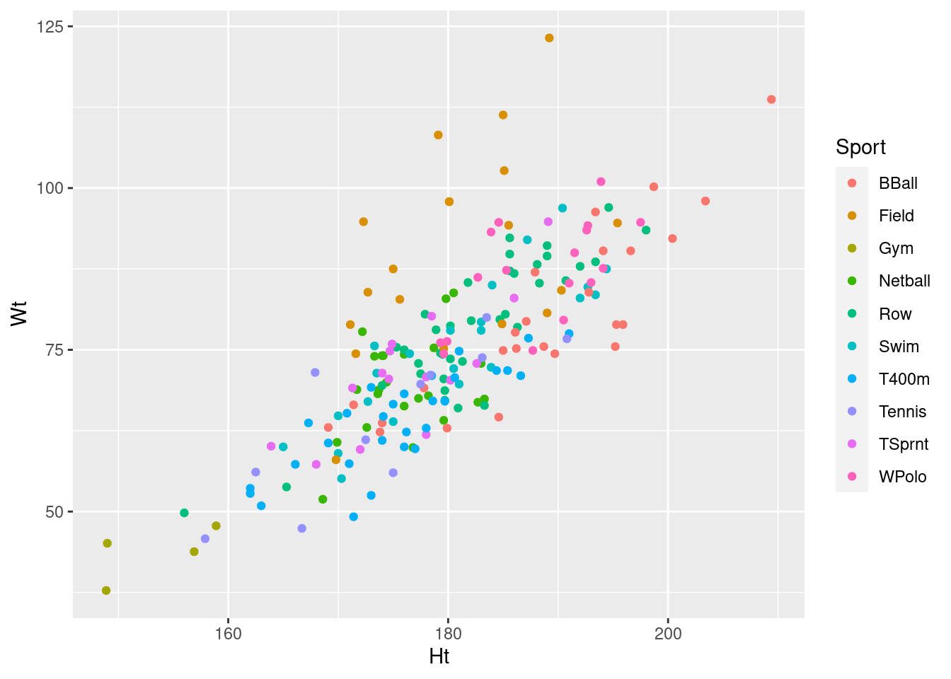

The reason for giving you the axes to use is (i) neither variable is really a response, so it doesn’t actually matter which one goes on which axis, and (ii) I wanted to give the grader something consistent to look at.

\(\blacksquare\)

Explain briefly why a multinomial model (multinom from nnet) would be the best thing to use to predict sport played from the other variables.

Solution

The categories of Sport are not in any kind of order, and there are more than two of them. That’s really all you needed, for which two marks was kind of generous.

\(\blacksquare\)

Fit a suitable model for predicting sport played from height and weight. (You don’t need to look at the results.) 100 steps isn’t quite enough, so set maxit equal to a larger number to allow the estimation to finish.

Solution

120 steps is actually enough, but any number larger than 110 is fine. It doesn’t matter if your guess is way too high. Like this:

library(nnet)
sport.1 <- multinom(Sport ~ Ht + Wt, data = athletes, maxit = 200)

## # weights:  40 (27 variable)
## initial  value 465.122189 
## iter  10 value 410.089598
## iter  20 value 391.426721
## iter  30 value 365.829150
## iter  40 value 355.326457
## iter  50 value 351.255395
## iter  60 value 350.876479
## iter  70 value 350.729699
## iter  80 value 350.532323
## iter  90 value 350.480130
## iter 100 value 350.349271
## iter 110 value 350.312029
## final  value 350.311949 
## converged

As long as you see the word converged at the end, you’re good.

\(\blacksquare\)

Demonstrate using anova that Wt should not be removed from this model.

Solution

The idea is to fit a model without Wt, and then show that it fits significantly worse. This converges in less than 100 iterations, so you can have maxit or not as you prefer:

sport.2 <- update(sport.1, . ~ . - Wt)

## # weights:  30 (18 variable)
## initial  value 465.122189 
## iter  10 value 447.375728
## iter  20 value 413.597441
## iter  30 value 396.685596
## iter  40 value 394.121380
## iter  50 value 394.116993
## iter  60 value 394.116434
## final  value 394.116429 
## converged

anova(sport.2, sport.1, test = "Chisq")

## Likelihood ratio tests of Multinomial Models
## 
## Response: Sport
##     Model Resid. df Resid. Dev   Test    Df LR stat.      Pr(Chi)
## 1      Ht      1800   788.2329                                   
## 2 Ht + Wt      1791   700.6239 1 vs 2     9 87.60896 4.884981e-15

The P-value is very small indeed, so the bigger model sport.1 is definitely better (or the smaller model sport.2 is significantly worse, however you want to say it). So taking Wt out is definitely a mistake.

This is what I would have guessed (I actually wrote the question in anticipation of this being the answer) because weight certainly seems to help in distinguishing the sports. For example, the field athletes seem to be heavy for their height compared to the other athletes (look back at the graph you made).

drop1, the obvious thing, doesn’t work here:

drop1(sport.1, test = "Chisq", trace = T)

## trying - Ht

## Error in if (trace) {: argument is not interpretable as logical

I gotta figure out what that error is. Does step?

step(sport.1, direction = "backward", test = "Chisq")

## Start:  AIC=754.62
## Sport ~ Ht + Wt
## 
## trying - Ht 
## # weights:  30 (18 variable)
## initial  value 465.122189 
## iter  10 value 441.367394
## iter  20 value 381.021649
## iter  30 value 380.326030
## final  value 380.305003 
## converged
## trying - Wt 
## # weights:  30 (18 variable)
## initial  value 465.122189 
## iter  10 value 447.375728
## iter  20 value 413.597441
## iter  30 value 396.685596
## iter  40 value 394.121380
## iter  50 value 394.116993
## iter  60 value 394.116434
## final  value 394.116429 
## converged
##        Df      AIC
## <none> 27 754.6239
## - Ht   18 796.6100
## - Wt   18 824.2329

## Call:
## multinom(formula = Sport ~ Ht + Wt, data = athletes, maxit = 200)
## 
## Coefficients:
##         (Intercept)         Ht          Wt
## Field      59.98535 -0.4671650  0.31466413
## Gym       112.49889 -0.5027056 -0.57087657
## Netball    47.70209 -0.2947852  0.07992763
## Row        35.90829 -0.2517942  0.14164007
## Swim       36.82832 -0.2444077  0.10544986
## T400m      32.73554 -0.1482589 -0.07830622
## Tennis     41.92855 -0.2278949 -0.01979877
## TSprnt     51.43723 -0.3359534  0.12378285
## WPolo      23.35291 -0.2089807  0.18819526
## 
## Residual Deviance: 700.6239 
## AIC: 754.6239

Curiously enough, it does. The final model is the same as the initial one, telling us that neither variable should be removed.

\(\blacksquare\)

Make a data frame consisting of all combinations of Ht 160, 180 and 200 (cm), and Wt 50, 75, and 100 (kg), and use it to obtain predicted probabilities of athletes of those heights and weights playing each of the sports. Display the results. You might have to display them smaller, or reduce the number of decimal places⁵¹ to fit them on the page.

Solution

To get all combinations of those heights and weights, use datagrid:

new <- datagrid(model = sport.1, Ht = c(160, 180, 200), Wt = c(50, 75, 100))
new

##     Ht  Wt
## 1: 160  50
## 2: 160  75
## 3: 160 100
## 4: 180  50
## 5: 180  75
## 6: 180 100
## 7: 200  50
## 8: 200  75
## 9: 200 100

(check: \(3 \times 3 = 9\) rows.)

Then predict:

p <- predictions(sport.1, newdata = new, type = "probs")
p

##    rowid  type   group    predicted std.error  Ht  Wt
## 1      1 probs   BBall 2.147109e-03         0 160  50
## 2      2 probs   BBall 1.044581e-04         0 160  75
## 3      3 probs   BBall 5.541050e-08         0 160 100
## 4      4 probs   BBall 9.142760e-02         0 180  50
## 5      5 probs   BBall 7.787300e-02         0 180  75
## 6      6 probs   BBall 5.379479e-04         0 180 100
## 7      7 probs   BBall 6.907544e-01         0 200  50
## 8      8 probs   BBall 8.889269e-01         0 200  75
## 9      9 probs   BBall 2.738448e-01         0 200 100
## 10     1 probs   Field 5.676191e-03         0 160  50
## 11     2 probs   Field 7.203893e-01         0 160  75
## 12     3 probs   Field 9.968725e-01         0 160 100
## 13     4 probs   Field 2.116103e-05         0 180  50
## 14     5 probs   Field 4.701849e-02         0 180  75
## 15     6 probs   Field 8.473139e-01         0 180 100
## 16     7 probs   Field 1.399715e-08         0 200  50
## 17     8 probs   Field 4.698989e-05         0 200  75
## 18     9 probs   Field 3.776290e-02         0 200 100
## 19     1 probs     Gym 7.269646e-02         0 160  50
## 20     2 probs     Gym 2.240720e-09         0 160  75
## 21     3 probs     Gym 7.530504e-19         0 160 100
## 22     4 probs     Gym 1.331347e-04         0 180  50
## 23     5 probs     Gym 7.184344e-11         0 180  75
## 24     6 probs     Gym 3.144321e-19         0 180 100
## 25     7 probs     Gym 4.326057e-08         0 200  50
## 26     8 probs     Gym 3.527126e-14         0 200  75
## 27     9 probs     Gym 6.884080e-21         0 200 100
## 28     1 probs Netball 1.997276e-01         0 160  50
## 29     2 probs Netball 7.166865e-02         0 160  75
## 30     3 probs Netball 2.804029e-04         0 160 100
## 31     4 probs Netball 2.339857e-02         0 180  50
## 32     5 probs Netball 1.469948e-01         0 180  75
## 33     6 probs Netball 7.489597e-03         0 180 100
## 34     7 probs Netball 4.863664e-04         0 200  50
## 35     8 probs Netball 4.616460e-03         0 200  75
## 36     9 probs Netball 1.048940e-02         0 200 100
## 37     1 probs     Row 3.205118e-02         0 160  50
## 38     2 probs     Row 5.379841e-02         0 160  75
## 39     3 probs     Row 9.845934e-04         0 160 100
## 40     4 probs     Row 8.871768e-03         0 180  50
## 41     5 probs     Row 2.607097e-01         0 180  75
## 42     6 probs     Row 6.213668e-02         0 180 100
## 43     7 probs     Row 4.357120e-04         0 200  50
## 44     8 probs     Row 1.934547e-02         0 200  75
## 45     9 probs     Row 2.056153e-01         0 200 100
## 46     1 probs    Swim 4.293546e-02         0 160  50
## 47     2 probs    Swim 2.916160e-02         0 160  75
## 48     3 probs    Swim 2.159577e-04         0 160 100
## 49     4 probs    Swim 1.377656e-02         0 180  50
## 50     5 probs    Swim 1.638165e-01         0 180  75
## 51     6 probs    Swim 1.579859e-02         0 180 100
## 52     7 probs    Swim 7.843113e-04         0 200  50
## 53     8 probs    Swim 1.409088e-02         0 200  75
## 54     9 probs    Swim 6.060159e-02         0 200 100
## 55     1 probs   T400m 3.517558e-01         0 160  50
## 56     2 probs   T400m 2.416185e-03         0 160  75
## 57     3 probs   T400m 1.809594e-07         0 160 100
## 58     4 probs   T400m 7.721547e-01         0 180  50
## 59     5 probs   T400m 9.285706e-02         0 180  75
## 60     6 probs   T400m 9.056685e-05         0 180 100
## 61     7 probs   T400m 3.007396e-01         0 200  50
## 62     8 probs   T400m 5.464293e-02         0 200  75
## 63     9 probs   T400m 2.376695e-03         0 200 100
## 64     1 probs  Tennis 1.885847e-01         0 160  50
## 65     2 probs  Tennis 5.592833e-03         0 160  75
## 66     3 probs  Tennis 1.808504e-06         0 160 100
## 67     4 probs  Tennis 8.418976e-02         0 180  50
## 68     5 probs  Tennis 4.371258e-02         0 180  75
## 69     6 probs  Tennis 1.840761e-04         0 180 100
## 70     7 probs  Tennis 6.668610e-03         0 200  50
## 71     8 probs  Tennis 5.231368e-03         0 200  75
## 72     9 probs  Tennis 9.824069e-04         0 200 100
## 73     1 probs  TSprnt 1.033315e-01         0 160  50
## 74     2 probs  TSprnt 1.109879e-01         0 160  75
## 75     3 probs  TSprnt 1.299813e-03         0 160 100
## 76     4 probs  TSprnt 5.313751e-03         0 180  50
## 77     5 probs  TSprnt 9.992310e-02         0 180  75
## 78     6 probs  TSprnt 1.523963e-02         0 180 100
## 79     7 probs  TSprnt 4.848339e-05         0 200  50
## 80     8 probs  TSprnt 1.377496e-03         0 200  75
## 81     9 probs  TSprnt 9.368804e-03         0 200 100
## 82     1 probs   WPolo 1.094045e-03         0 160  50
## 83     2 probs   WPolo 5.880674e-03         0 160  75
## 84     3 probs   WPolo 3.446523e-04         0 160 100
## 85     4 probs   WPolo 7.129763e-04         0 180  50
## 86     5 probs   WPolo 6.709478e-02         0 180  75
## 87     6 probs   WPolo 5.120898e-02         0 180 100
## 88     7 probs   WPolo 8.244005e-05         0 200  50
## 89     8 probs   WPolo 1.172154e-02         0 200  75
## 90     9 probs   WPolo 3.989581e-01         0 200 100

I saved these, because I want to talk about what to do next. The normal procedure is to say that there is a prediction for each group (sport), so we want to grab only the columns we need and pivot wider. But, this time there are 10 sports (see how there are \(9 \times 10 = 90\) rows, with a predicted probability for each height-weight combo for each sport). I suggested reducing the number of decimal places in the predictions; the time to do that is now, while they are all in one column (rather than trying to round a bunch of columns all at once, which is doable but more work). Hence:

p %>% 
  mutate(predicted = round(predicted, 2)) %>% 
  select(group, predicted, Ht, Wt) %>% 
  pivot_wider(names_from = group, values_from = predicted)

## # A tibble: 9 × 12
##      Ht    Wt BBall Field   Gym Netball   Row  Swim T400m Tennis TSprnt WPolo
##   <dbl> <dbl> <dbl> <dbl> <dbl>   <dbl> <dbl> <dbl> <dbl>  <dbl>  <dbl> <dbl>
## 1   160    50  0     0.01  0.07    0.2   0.03  0.04  0.35   0.19   0.1   0   
## 2   160    75  0     0.72  0       0.07  0.05  0.03  0      0.01   0.11  0.01
## 3   160   100  0     1     0       0     0     0     0      0      0     0   
## 4   180    50  0.09  0     0       0.02  0.01  0.01  0.77   0.08   0.01  0   
## 5   180    75  0.08  0.05  0       0.15  0.26  0.16  0.09   0.04   0.1   0.07
## 6   180   100  0     0.85  0       0.01  0.06  0.02  0      0      0.02  0.05
## 7   200    50  0.69  0     0       0     0     0     0.3    0.01   0     0   
## 8   200    75  0.89  0     0       0     0.02  0.01  0.05   0.01   0     0.01
## 9   200   100  0.27  0.04  0       0.01  0.21  0.06  0      0      0.01  0.4

This works (although even then it might not all fit onto the page and you’ll have to scroll left and right to see everything).

If you forget to round until the end, you’ll have to do something like this:

p %>% 
  select(group, predicted, Ht, Wt) %>% 
  pivot_wider(names_from = group, values_from = predicted) %>% 
  mutate(across(BBall:WPolo, ~round(., 2)))

## # A tibble: 9 × 12
##      Ht    Wt BBall Field   Gym Netball   Row  Swim T400m Tennis TSprnt WPolo
##   <dbl> <dbl> <dbl> <dbl> <dbl>   <dbl> <dbl> <dbl> <dbl>  <dbl>  <dbl> <dbl>
## 1   160    50  0     0.01  0.07    0.2   0.03  0.04  0.35   0.19   0.1   0   
## 2   160    75  0     0.72  0       0.07  0.05  0.03  0      0.01   0.11  0.01
## 3   160   100  0     1     0       0     0     0     0      0      0     0   
## 4   180    50  0.09  0     0       0.02  0.01  0.01  0.77   0.08   0.01  0   
## 5   180    75  0.08  0.05  0       0.15  0.26  0.16  0.09   0.04   0.1   0.07
## 6   180   100  0     0.85  0       0.01  0.06  0.02  0      0      0.02  0.05
## 7   200    50  0.69  0     0       0     0     0     0.3    0.01   0     0   
## 8   200    75  0.89  0     0       0     0.02  0.01  0.05   0.01   0     0.01
## 9   200   100  0.27  0.04  0       0.01  0.21  0.06  0      0      0.01  0.4

In words, “for each column from BBall through WPolo, replace it by itself rounded to 2 decimals”.

There’s nothing magic about two decimals; three or maybe even four would be fine. A small enough number that you can see most or all of the columns at once, and easily compare the numbers for size (which is hard when some of them are in scientific notation).

Extra: you can even abbreviate the sport names, like this:

p %>% 
  mutate(predicted = round(predicted, 2),
         group = abbreviate(group, 3)) %>% 
  select(group, predicted, Ht, Wt) %>% 
  pivot_wider(names_from = group, values_from = predicted)

## # A tibble: 9 × 12
##      Ht    Wt   BBl   Fld   Gym   Ntb   Row   Swm   T40   Tnn   TSp   WPl
##   <dbl> <dbl> <dbl> <dbl> <dbl> <dbl> <dbl> <dbl> <dbl> <dbl> <dbl> <dbl>
## 1   160    50  0     0.01  0.07  0.2   0.03  0.04  0.35  0.19  0.1   0   
## 2   160    75  0     0.72  0     0.07  0.05  0.03  0     0.01  0.11  0.01
## 3   160   100  0     1     0     0     0     0     0     0     0     0   
## 4   180    50  0.09  0     0     0.02  0.01  0.01  0.77  0.08  0.01  0   
## 5   180    75  0.08  0.05  0     0.15  0.26  0.16  0.09  0.04  0.1   0.07
## 6   180   100  0     0.85  0     0.01  0.06  0.02  0     0     0.02  0.05
## 7   200    50  0.69  0     0     0     0     0     0.3   0.01  0     0   
## 8   200    75  0.89  0     0     0     0.02  0.01  0.05  0.01  0     0.01
## 9   200   100  0.27  0.04  0     0.01  0.21  0.06  0     0     0.01  0.4

Once again, the time to do this is while everything is long, so that you only have one column to work with.⁵² Again, you can do this at the end, but it’s more work, because you are now renaming columns:

p %>% 
  mutate(predicted = round(predicted, 2)) %>% 
  select(group, predicted, Ht, Wt) %>% 
  pivot_wider(names_from = group, values_from = predicted) %>% 
  rename_with(~abbreviate(., 3), everything())

## # A tibble: 9 × 12
##      Ht    Wt   BBl   Fld   Gym   Ntb   Row   Swm   T40   Tnn   TSp   WPl
##   <dbl> <dbl> <dbl> <dbl> <dbl> <dbl> <dbl> <dbl> <dbl> <dbl> <dbl> <dbl>
## 1   160    50  0     0.01  0.07  0.2   0.03  0.04  0.35  0.19  0.1   0   
## 2   160    75  0     0.72  0     0.07  0.05  0.03  0     0.01  0.11  0.01
## 3   160   100  0     1     0     0     0     0     0     0     0     0   
## 4   180    50  0.09  0     0     0.02  0.01  0.01  0.77  0.08  0.01  0   
## 5   180    75  0.08  0.05  0     0.15  0.26  0.16  0.09  0.04  0.1   0.07
## 6   180   100  0     0.85  0     0.01  0.06  0.02  0     0     0.02  0.05
## 7   200    50  0.69  0     0     0     0     0     0.3   0.01  0     0   
## 8   200    75  0.89  0     0     0     0.02  0.01  0.05  0.01  0     0.01
## 9   200   100  0.27  0.04  0     0.01  0.21  0.06  0     0     0.01  0.4

rename doesn’t work with across (you will get an error if you try it), so you need to use rename_with⁵³. This has syntax “how to rename” first (here, with an abbreviated version of itself), and “what to rename” second (here, everything, or BBall through WPolo if you prefer).

\(\blacksquare\)

For an athlete who is 180 cm tall and weighs 100 kg, what sport would you guess they play? How sure are you that you are right? Explain briefly.

Solution

Find this height and weight in your predictions (it’s row 6). Look along the line for the highest probability, which is 0.85 for Field (that is, field athletics). All the other probabilities are much smaller (the biggest of the others is 0.06). So this means we would guess the athlete to be a field athlete, and because the predicted probability is so big, we are very likely to be right. This kind of thought process is characteristic of discriminant analysis, which we’ll see more of later in the course. Compare that with the scatterplot you drew earlier: the field athletes do seem to be distinct from the rest in terms of height-weight combination. Some of the other height-weight combinations are almost equally obvious: for example, very tall people who are not very heavy are likely to play basketball. 400m runners are likely to be of moderate height but light weight. Some of the other sports, or height-weight combinations, are difficult to judge. Consider also that we have mixed up males and females in this data set. We might gain some clarity by including Sex in the model, and also in the predictions. But I wanted to keep this question relatively simple for you, and I wanted to stop from getting unreasonably long. (You can decide whether you think it’s already too long.)

\(\blacksquare\)

For this, use round.↩︎
If you do not take out the NA values, they are shown separately on the end of the summary for that column.↩︎
The American Green party is more libertarian than Green parties elsewhere.↩︎
Northern Ireland’s political parties distinguish themselves by politics and religion. Northern Ireland has always had political tensions between its Protestants and its Catholics.↩︎
There are three political parties; using the first as a baseline, there are therefore \(3-1=2\) coefficients for each variable.↩︎
It amuses me that Toronto’s current (2021) mayor, named Tory, is politically a Tory.↩︎
When you have variables that are categories, you might have more than one individual with exactly the same categories; on the other hand, if they had measured Size as, say, length in centimetres, it would have been very unlikely to get two alligators of exactly the same size.↩︎
Discovered by me two minutes ago.↩︎
Just don’t use a measure of spread, which will give you zero.↩︎
There were only 216 alligators total, which is a small sample size for this kind of thing, especially with all those parameters to estimate.↩︎
Better, because it doesn’t do predictions for all the other districts as well, only to throw them away, which is what we did above. When the predictions take so long, it’s worth trying to speed it up.↩︎
I know I just said not to do this kind of thing, but counting is really fast, while unnecessary predictions are really slow.↩︎
There is only one district, so we can just put that in here.↩︎
The same thing applies if you are doing something like webscraping, that is to say downloading stuff from the web that you then want to do something with. Download it once and save it, then you can take as long as you need to decide what you’re doing with it.↩︎
Statistical significance as an idea grew up in the days before “big data”.↩︎
For this, use round.↩︎
abbreviate comes from base R; it returns an abbreviated version of its (text) input, with a minimum length of its second input. If two abbreviations come out the same, it makes them longer until they are different. It has some heuristics to get things short enough: remove vowels, then remove letters on the end.↩︎
Which I learned about today.↩︎