29 Logistic regression with nominal response

library(nnet)
library(tidyverse)

29.1 Finding non-missing values

* This is to prepare you for something in the next question. It’s meant to be easy.

In R, the code NA stands for “missing value” or “value not known”. In R, NA should not have quotes around it. (It is a special code, not a piece of text.)

Create a vector v that contains some numbers and some missing values, using c(). Put those values into a one-column data frame.
Obtain a new column containing is.na(v). When is this true and when is this false?
The symbol ! means “not” in R (and other programming languages). What does !is.na(v) do? Create a new column containing that.
Use filter to display just the rows of your data frame that have a non-missing value of v.

29.2 European Social Survey and voting

The European Social Survey is a giant survey carried out across Europe covering demographic information, attitudes to and amount of education, politics and so on. In this question, we will investigate what might make British people vote for a certain political party.

The information for this question is in a (large) spreadsheet at link. There is also a “codebook” at link that tells you what all the variables are. The ones we will use are the last five columns of the spreadsheet, described on pages 11 onwards of the codebook. (I could have given you more, but I didn’t want to make this any more complicated than it already was.)

Read in the .csv file, and verify that you have lots of rows and columns.
* Use the codebook to find out what the columns prtvtgb, gndr, agea, eduyrs and inwtm are. What do the values 1 and 2 for gndr mean? (You don’t, at this point, have to worry about the values for the other variables.)
The three major political parties in Britain are the Conservative, Labour and Liberal Democrat. (These, for your information, correspond roughly to the Canadian Progressive Conservative, NDP and Liberal parties.) For the variable that corresponds to “political party voted for at the last election”, which values correspond to these three parties?
Normally, I would give you a tidied-up data set. But I figure you could use some practice tidying this one up. As the codebook shows, there are some numerical codes for missing values, and we want to omit those. We want just the columns prtvtgb through inwtm from the right side of the spreadsheet. Use dplyr or tidyr tools to (i) select only these columns, (ii) include the rows that correspond to people who voted for one of the three major parties, (iii) include the rows that have an age at interview less than 999, (iv) include the rows that have less than 40 years of education, (v) include the rows that are not missing on inwtm (use the idea from Question~here for (v)). The last four of those (the inclusion of rows) can be done in one go.
Why is my response variable nominal rather than ordinal? How can I tell? Which R function should I use, therefore, to fit my model?
* Take the political party voted for, and turn it into a factor, by feeding it into factor. Fit an appropriate model to predict political party voted for at the last election (as a factor) from all the other variables. Gender is really a categorical variable too, but since there are only two possible values it can be treated as a number.
We have a lot of explanatory variables. The standard way to test whether we need all of them is to take one of them out at a time, and test which ones we can remove. This is a lot of work. We won’t do that. Instead, the R function step does what you want. You feed step two things: a fitted model object, and the option trace=0 (otherwise you get a lot of output). The final part of the output from step tells you which explanatory variables you need to keep. Run step on your fitted model. Which explanatory variables need to stay in the model here?
Fit the model indicated by step (in the last part).
I didn’t think that interview length could possibly be relevant to which party a person voted for. Test whether interview length can be removed from your model of the last part. What do you conclude? (Note that step and this test may disagree.)
Use your best model to obtain predictions from some suitably chosen combinations of values of the explanatory variables that remain. (If you have quantitative explanatory variables left, you could use their first and third quartiles as values to predict from. Running summary on the data frame will get summaries of all the variables.)
What is the effect of increasing age? What is the effect of an increase in years of education?

29.3 Alligator food

What do alligators most like to eat? 219 alligators were captured in four Florida lakes. Each alligator’s stomach contents were observed, and the food that the alligator had eaten was classified into one of five categories: fish, invertebrates (such as snails or insects), reptiles (such as turtles), birds, and “other” (such as amphibians, plants or rocks). The researcher noted for each alligator what that alligator had most of in its stomach, as well as the gender of each alligator and whether it was “large” or “small” (greater or less than 2.3 metres in length). The data can be found in link. The numbers in the data set (apart from the first column) are all frequencies. (You can ignore that first column “profile”.)

Our aim is to predict food type from the other variables.

Read in the data and display the first few lines. Describe how the data are not “tidy”.
Use pivot_longer to arrange the data suitably for analysis (which will be using multinom). Demonstrate (by looking at the first few rows of your new data frame) that you now have something tidy.
What is different about this problem, compared to Question here, that would make multinom the right tool to use?
Fit a suitable multinomial model predicting food type from gender, size and lake. Does each row represent one alligator or more than one? If more than one, account for this in your modelling.
Do a test to see whether Gender should stay in the model. (This will entail fitting another model.) What do you conclude?
Predict the probability that an alligator prefers each food type, given its size, gender (if necessary) and the lake it was found in, using the more appropriate of the two models that you have fitted so far. This means (i) making a data frame for prediction, and (ii) obtaining and displaying the predicted probabilities in a way that is easy to read.
What do you think is the most important way in which the lakes differ? (Hint: look at where the biggest predicted probabilities are.)
How would you describe the major difference between the diets of the small and large alligators?

29.4 Crimes in San Francisco

The data in link is a subset of a huge dataset of crimes committed in San Francisco between 2003 and 2015. The variables are:

Dates: the date and time of the crime
Category: the category of crime, eg. “larceny” or “vandalism” (response).
Descript: detailed description of crime.
DayOfWeek: the day of the week of the crime.
PdDistrict: the name of the San Francisco Police Department district in which the crime took place.
Resolution: how the crime was resolved
Address: approximate street address of crime
X: longitude
Y: latitude

Our aim is to see whether the category of crime depends on the day of the week and the district in which it occurred. However, there are a lot of crime categories, so we will focus on the top four “interesting” ones, which are the ones included in this data file.

Some of the model-fitting takes a while (you’ll see why below). In your Quarto document, you can wait for the models to fit each time you re-run your document, or you can insert #| cache: true below the top line of your code chunk (above the first line of actual code). What that does is to re-run that code chunk only if it changes; if it hasn’t changed it will use the saved results from last time it was run. That can save you a lot of waiting around.

Read in the data and display the dataset (or, at least, part of it).
Fit a multinomial logistic regression that predicts crime category from day of week and district. (You don’t need to look at it.) The model-fitting produces some output in the console to convince you that it has worked.
Fit a model that predicts Category from only the district. Hand in the output from the fitting process as well.
Use anova to compare the two models you just obtained. What does the anova tell you?
Using your preferred model, obtain predicted probabilities that a crime will be of each of these four categories for each day of the week in the TENDERLOIN district (the name is ALL CAPS). This will mean constructing a data frame to predict from, obtaining the predictions and then displaying them suitably.
Describe briefly how the weekend days Saturday and Sunday differ from the rest.

29.5 Crimes in San Francisco – the data

The data in link is a huge dataset of crimes committed in San Francisco between 2003 and 2015. The variables are:

Dates: the date and time of the crime
Category: the category of crime, eg. “larceny” or “vandalism” (response).
Descript: detailed description of crime.
DayOfWeek: the day of the week of the crime.
PdDistrict: the name of the San Francisco Police Department district in which the crime took place.
Resolution: how the crime was resolved
Address: approximate street address of crime
X: longitude
Y: latitude

Read in the data and verify that you have these columns and a lot of rows. (The data may take a moment to read in. You will see why.)
How is the response variable here different to the one in the question about steak preferences (and therefore why would multinom from package nnet be the method of choice)?
Find out which crime categories there are, and arrange them in order of how many crimes there were in each category.
Which are the four most frequent “interesting” crime categories, that is to say, not including “other offenses” and “non-criminal”? Get them into a vector called my.crimes. See if you can find a way of doing this that doesn’t involve typing them in (for full marks).
(Digression, but needed for the next part.) The R vector letters contains the lowercase letters from a to z. Consider the vector ('a','m',3,'Q'). Some of these are found amongst the lowercase letters, and some not. Type these into a vector v and explain briefly why v %in% letters produces what it does.
We are going to filter only the rows of our data frame that have one of the crimes in my.crimes as their Category. Also, select only the columns Category, DayOfWeek and PdDistrict. Save the resulting data frame and display its structure. (You should have a lot fewer rows than you did before.)
Save these data in a file sfcrime1.csv.

29.6 What sports do these athletes play?

The data at link are physical and physiological measurements of 202 male and female Australian elite athletes. The data values are separated by tabs. We are going to see whether we can predict the sport an athlete plays from their height and weight.

The sports, if you care, are respectively basketball, “field athletics” (eg. shot put, javelin throw, long jump etc.), gymnastics, netball, rowing, swimming, 400m running, tennis, sprinting (100m or 200m running), water polo.

Read in the data and display the first few rows.
Make a scatterplot of height vs. weight, with the points coloured by what sport the athlete plays. Put height on the \(x\)-axis and weight on the \(y\)-axis.
Explain briefly why a multinomial model (multinom from nnet) would be the best thing to use to predict sport played from the other variables.
Fit a suitable model for predicting sport played from height and weight. (You don’t need to look at the results.) 100 steps isn’t quite enough, so set maxit equal to a larger number to allow the estimation to finish.
Demonstrate using anova that Wt should not be removed from this model.
Make a data frame consisting of all combinations of Ht 160, 180 and 200 (cm), and Wt 50, 75, and 100 (kg), and use it to obtain predicted probabilities of athletes of those heights and weights playing each of the sports. Display the results. You might have to display them smaller, or reduce the number of decimal places¹ to fit them on the page.
For an athlete who is 180 cm tall and weighs 100 kg, what sport would you guess they play? How sure are you that you are right? Explain briefly.

My solutions follow:

29.7 Finding non-missing values

* This is to prepare you for something in the next question. It’s meant to be easy.

In R, the code NA stands for “missing value” or “value not known”. In R, NA should not have quotes around it. (It is a special code, not a piece of text.)

Create a vector v that contains some numbers and some missing values, using c(). Put those values into a one-column data frame.

Solution

Like this. The arrangement of numbers and missing values doesn’t matter, as long as you have some of each:

v <- c(1, 2, NA, 4, 5, 6, 9, NA, 11)
mydata <- tibble(v)
mydata

This has one column called v.

\(\blacksquare\)

Obtain a new column containing is.na(v). When is this true and when is this false?

Solution

mydata <- mydata %>% mutate(isna = is.na(v))
mydata

This is TRUE if the corresponding element of v is missing (in my case, the third value and the second-last one), and FALSE otherwise (when there is an actual value there).

\(\blacksquare\)

The symbol ! means “not” in R (and other programming languages). What does !is.na(v) do? Create a new column containing that.

Solution

Try it and see. Give it whatever name you like. My name reflects that I know what it’s going to do:

mydata <- mydata %>% mutate(notisna = !is.na(v))
mydata

This is the logical opposite of is.na: it’s true if there is a value, and false if it’s missing.

\(\blacksquare\)

Use filter to display just the rows of your data frame that have a non-missing value of v.

Solution

filter takes a column to say which rows to pick, in which case the column should contain something that either is TRUE or FALSE, or something that can be interpreted that way:

mydata %>% filter(notisna)

or you can provide filter something that can be calculated from what’s in the data frame, and also returns something that is either true or false:

mydata %>% filter(!is.na(v))

In either case, I only have non-missing values of v.

\(\blacksquare\)

29.8 European Social Survey and voting

Read in the .csv file, and verify that you have lots of rows and columns.

Solution

The obvious way. Printing it out will display some of the data and tell you how many rows and columns you have:

my_url <- "http://ritsokiguess.site/datafiles/ess.csv"
ess <- read_csv(my_url)

Rows: 2286 Columns: 17
── Column specification ────────────────────────────────────────────────────────
Delimiter: ","
chr  (4): cntry, cname, cproddat, name
dbl (13): cedition, cseqno, essround, edition, idno, dweight, pspwght, pweig...

ℹ Use `spec()` to retrieve the full column specification for this data.
ℹ Specify the column types or set `show_col_types = FALSE` to quiet this message.

ess

2286 rows and 17 columns.

\(\blacksquare\)

* Use the codebook to find out what the columns prtvtgb, gndr, agea, eduyrs and inwtm are. What do the values 1 and 2 for gndr mean? (You don’t, at this point, have to worry about the values for the other variables.)

Solution

Respectively, political party voted for at last election, gender (of respondent), age at interview, years of full-time education, length of interview (in minutes). For gndr, male is 1 and female is 2.

\(\blacksquare\)

The three major political parties in Britain are the Conservative, Labour and Liberal Democrat. (These, for your information, correspond roughly to the Canadian Progressive Conservative, NDP and Liberal parties.) For the variable that corresponds to “political party voted for at the last election”, which values correspond to these three parties?

Solution

1, 2 and 3 respectively. (That was easy!)

\(\blacksquare\)

Normally, I would give you a tidied-up data set. But I figure you could use some practice tidying this one up. As the codebook shows, there are some numerical codes for missing values, and we want to omit those. We want just the columns prtvtgb through inwtm from the right side of the spreadsheet. Use dplyr or tidyr tools to (i) select only these columns, (ii) include the rows that correspond to people who voted for one of the three major parties, (iii) include the rows that have an age at interview less than 999, (iv) include the rows that have less than 40 years of education, (v) include the rows that are not missing on inwtm (use the idea from Question~here for (v)). The last four of those (the inclusion of rows) can be done in one go.

Solution

The major parties are numbered 1, 2 and 3, so we can select the ones less than 4 (or <=3). The reference back to the last question is a hint to use !is.na(). It also works to use drop_na, if you are familiar with that.

ess %>%
  select(prtvtgb:inwtm) %>%
  filter(prtvtgb < 4, agea < 999, eduyrs < 40, !is.na(inwtm)) -> ess.major

You might get a weird error in select, something about “unused argument”. If this happens to you, it’s not because you used select wrong, it’s because you used the wrong select! There is one in MASS, and you need to make sure that this package is “detached” so that you use the select you want, namely the one in dplyr, loaded with the tidyverse. Use the instructions at the end of the mobile phones question or the abortion question to do this.

The other way around this is to say, instead of select, dplyr::select with two colons. This means “the select that lives in dplyr, no other”, and is what Wikipedia calls “disambiguation”: out of several things with the same name, you say which one you mean.

If you do the pipeline, you will probably not get it right the first time. (I didn’t.) For debugging, try out one step at a time, and summarize what you have so far, so that you can check it for correctness. A handy trick for that is to make the last piece of your pipeline summary(), which produces a summary of the columns of the resulting data frame. For example, I first did this (note that my filter is a lot simpler than the one above):

ess %>%
  select(prtvtgb:inwtm) %>%
  filter(prtvtgb < 4, !is.na(inwtm)) %>%
  summary()

    prtvtgb           gndr            agea            eduyrs     
 Min.   :1.000   Min.   :1.000   Min.   : 18.00   Min.   : 0.00  
 1st Qu.:1.000   1st Qu.:1.000   1st Qu.: 44.00   1st Qu.:11.00  
 Median :2.000   Median :2.000   Median : 58.00   Median :13.00  
 Mean   :1.803   Mean   :1.572   Mean   : 61.74   Mean   :14.23  
 3rd Qu.:2.000   3rd Qu.:2.000   3rd Qu.: 71.00   3rd Qu.:16.00  
 Max.   :3.000   Max.   :2.000   Max.   :999.00   Max.   :88.00  
     inwtm       
 Min.   :  7.00  
 1st Qu.: 35.00  
 Median : 41.00  
 Mean   : 43.54  
 3rd Qu.: 50.00  
 Max.   :160.00

The mean of a categorical variable like party voted for or gender doesn’t make much sense, but it looks as if all the values are sensible ones (1 to 3 and 1, 2 respectively). However, the maximum values of age and years of education look like missing value codes, hence the other requirements I put in the question.²

Displaying as the last step of your pipeline also works, but the advantage of summary is that you get to see whether there are any unusual values, in this case unusually large values that are missing value codes.

\(\blacksquare\)

Why is my response variable nominal rather than ordinal? How can I tell? Which R function should I use, therefore, to fit my model?

Solution

The response variable is political party voted for. There is no (obvious) ordering to this (unless you want to try to place the parties on a left-right spectrum), so this is nominal, and you’ll need multinom from package nnet.

If I had included the minor parties and you were working on a left-right spectrum, you would have had to decide where to put the somewhat libertarian Greens³ or the parties that exist only in Northern Ireland.⁴

\(\blacksquare\)

* Take the political party voted for, and turn it into a factor, by feeding it into factor. Fit an appropriate model to predict political party voted for at the last election (as a factor) from all the other variables. Gender is really a categorical variable too, but since there are only two possible values it can be treated as a number.

Solution

This, or something like it. multinom lives in package nnet, which you’ll have to install first if you haven’t already:

library(nnet)
ess.1 <- multinom(factor(prtvtgb) ~ gndr + agea + eduyrs + inwtm, data = ess.major)

# weights:  18 (10 variable)
initial  value 1343.602829 
iter  10 value 1256.123798
final  value 1247.110080 
converged

Or create a factor version of your response in the data frame first:

ess.major <- ess.major %>% mutate(party = factor(prtvtgb))

and then:

ess.1a <- multinom(party ~ gndr + agea + eduyrs + inwtm, data = ess.major)

# weights:  18 (10 variable)
initial  value 1343.602829 
iter  10 value 1256.123798
final  value 1247.110080 
converged

\(\blacksquare\)

We have a lot of explanatory variables. The standard way to test whether we need all of them is to take one of them out at a time, and test which ones we can remove. This is a lot of work. We won’t do that. Instead, the R function step does what you want. You feed step two things: a fitted model object, and the option trace=0 (otherwise you get a lot of output). The final part of the output from step tells you which explanatory variables you need to keep. Run step on your fitted model. Which explanatory variables need to stay in the model here?

Solution

I tried to give you lots of hints here:

ess.2a <- step(ess.1, trace = 0)

trying - gndr 
trying - agea 
trying - eduyrs 
trying - inwtm 
# weights:  15 (8 variable)
initial  value 1343.602829 
iter  10 value 1248.343563
final  value 1248.253638 
converged
trying - agea 
trying - eduyrs 
trying - inwtm

ess.2a

Call:
multinom(formula = factor(prtvtgb) ~ agea + eduyrs + inwtm, data = ess.major)

Coefficients:
  (Intercept)        agea     eduyrs       inwtm
2    1.632266 -0.02153694 -0.0593757 0.009615167
3   -1.281031 -0.01869263  0.0886487 0.009337084

Residual Deviance: 2496.507 
AIC: 2512.507

If you didn’t save your output in a variable, you’ll get my last bit automatically.

The end of the output gives us coefficients for (and thus tells us we need to keep) age, years of education and interview length.

The actual numbers don’t mean much; it’s the indication that the variable has stayed in the model that makes a difference.⁵

If you’re wondering about the process: first step tries to take out each explanatory variable, one at a time, from the starting model (the one that contains all the variables). Then it finds the best model out of those and fits it. (It doesn’t tell us which model this is, but evidently it’s the one without gender.) Then it takes that model and tries to remove its explanatory variables one at a time (there are only three of them left). Having decided it cannot remove any of them, it stops, and shows us what’s left.

Leaving out the trace=0 shows more output and more detail on the process, but I figured this was enough (and this way, you don’t have to wade through all of that output). Try values like 1 or 2 for trace and see what you get.

\(\blacksquare\)

Fit the model indicated by step (in the last part).

Solution

Copy and paste, and take out the variables you don’t need. Or, better, save the output from step in a variable. This then becomes a fitted model object and you can look at it any of the ways you can look at a model fit. I found that gender needed to be removed, but if yours is different, follow through with whatever your step said to do.

ess.2 <- multinom(party ~ agea + eduyrs + inwtm, data = ess.major)

# weights:  15 (8 variable)
initial  value 1343.602829 
iter  10 value 1248.343563
final  value 1248.253638 
converged

If you saved the output from step, you’ll already have this and you don’t need to do it again:

anova(ess.2, ess.2a)

Same model.

\(\blacksquare\)

I didn’t think that interview length could possibly be relevant to which party a person voted for. Test whether interview length can be removed from your model of the last part. What do you conclude? (Note that step and this test may disagree.)

Solution

Fit the model without inwtm:

ess.3 <- multinom(party ~ agea + eduyrs, data = ess.major)

# weights:  12 (6 variable)
initial  value 1343.602829 
iter  10 value 1250.418281
final  value 1250.417597 
converged

and then use anova to compare them:

anova(ess.3, ess.2)

The P-value, 0.1149, is not small, which says that the smaller model is good, ie. the one without interview length.

I thought drop1 would also work here, but it appears not to:

drop1(ess.1, test = "Chisq")

trying - gndr

Error in if (trace) {: argument is not interpretable as logical

I think that’s a bug in multinom, since normally if step works, then drop1 will work too (normally step uses drop1).

The reason for the disagreement between step and anova is that step will tend to keep marginal explanatory variables, that is, ones that are “potentially interesting” but whose P-values might not be less than 0.05. There is still no substitute for your judgement in figuring out what to do! step uses a thing called AIC to decide what to do, rather than actually doing a test. If you know about “adjusted R-squared” in choosing explanatory variables for a regression, it’s the same idea: a variable can be not quite significant but still make the adjusted R-squared go up (typically only a little).

\(\blacksquare\)

Use your best model to obtain predictions from some suitably chosen combinations of values of the explanatory variables that remain. (If you have quantitative explanatory variables left, you could use their first and third quartiles as values to predict from. Running summary on the data frame will get summaries of all the variables.)

Solution

First make our new data frame of values to predict from. You can use quantile or summary to find the quartiles. I only had agea and eduyrs left, having decided that interview time really ought to come out:

summary(ess.major)

    prtvtgb           gndr            agea           eduyrs     
 Min.   :1.000   Min.   :1.000   Min.   :18.00   Min.   : 0.00  
 1st Qu.:1.000   1st Qu.:1.000   1st Qu.:44.00   1st Qu.:11.00  
 Median :2.000   Median :2.000   Median :58.00   Median :13.00  
 Mean   :1.803   Mean   :1.574   Mean   :57.19   Mean   :13.45  
 3rd Qu.:2.000   3rd Qu.:2.000   3rd Qu.:71.00   3rd Qu.:16.00  
 Max.   :3.000   Max.   :2.000   Max.   :94.00   Max.   :33.00  
     inwtm       party  
 Min.   :  7.0   1:484  
 1st Qu.: 35.0   2:496  
 Median : 41.0   3:243  
 Mean   : 43.7          
 3rd Qu.: 50.0          
 Max.   :160.0

Quartiles for age are 44 and 71, and for years of education are 11 and 16.

This time, instead of predicting for variable values that predictions chooses for us (like a five-number summary), we are predicting for “custom” values, ones that we chose. To set that up, the marginaleffects way is to use datagrid like this:

new <- datagrid(model = ess.3, agea = c(44, 71), eduyrs = c(11, 16))
new

What datagrid does is to make all combinations of your variable values, and along with that, to use “typical” values for the others: the mean, in the case of quantitative variables like inwtm, and the most common category for categorical ones like party. If you feed datagrid a model first, it only includes variables in that model, which is easier to make sense of:

datagrid(newdata = ess.major, agea = c(44, 71), eduyrs = c(11, 16))

The other variables don’t make much sense, since they are really categorical but expressed as numbers, but they are not in the best model, so that doesn’t do any harm. (In other cases, you might need to be more careful.)

Next, we feed this into predictions, using the above dataframe as newdata, and with our best model, ess.3 (the one without interview length). The results might confuse you at first, since you will probably get an error:

cbind(predictions(ess.3, newdata = new))

The error message gives you a hint about what to do: add a type = "probs" to predictions (which is a consequence of how multinom works):

cbind(predictions(ess.3, newdata = new, type = "probs"))

There are twelve rows for our four predictions, because there are three predictions for each of our four “people”: the probabilities of each one voting for each of the three parties. The party predicted for is in the column group, and the probability of each person (labelled by rowid) voting for that party is in predicted. Let’s simplify things by keeping only those columns and the ones we are predicting for:

cbind(predictions(ess.3, newdata = new, type = "probs")) %>% 
  select(rowid, group, estimate, agea, eduyrs)

and then pivot wider to get all three predictions for each person on one line:

cbind(predictions(ess.3, newdata = new, type = "probs")) %>% 
  select(rowid, group, estimate, agea, eduyrs) %>% 
  pivot_wider(names_from = group, values_from = estimate)

\(\blacksquare\)

What is the effect of increasing age? What is the effect of an increase in years of education?

Solution

To assess the effect of age, hold years of education constant. Thus, compare lines 1 and 3 (or 2 and 4): increasing age tends to increase the chance that a person will vote Conservative (party 1), and decrease the chance that a person will vote Labour (party 2). There doesn’t seem to be much effect of age on the chance that a person will vote Liberal Democrat.

To assess education, hold age constant, and thus compare rows 1 and 2 (or rows 3 and 4). This time, there isn’t much effect on the chances of voting Conservative, but as education increases, the chance of voting Labour goes down, and the chance of voting Liberal Democrat goes up.

A little history: back 150 or so years ago, Britain had two political parties, the Tories and the Whigs. The Tories became the Conservative party (and hence, in Britain and in Canada, the Conservatives are nicknamed Tories⁶). The Whigs became Liberals. At about the same time as working people got to vote (not women, yet, but working men) the Labour Party came into existence. The Labour Party has always been affiliated with working people and trades unions, like the NDP here. But power has typically alternated between Conservative and Labour goverments, with the Liberals as a third party. In the 1980s a new party called the Social Democrats came onto the scene, but on realizing that they couldn’t make much of a dent by themselves, they merged with the Liberals to form the Liberal Democrats, which became a slightly stronger third party.

I was curious about what the effect of interview length would be. Presumably, the effect is small, but I have no idea which way it would be. To assess this, this is predictions again, but this time we can let predictions pick some values for inwtm for us, and leave everything else at their mean. We have to remember to use the model ess.2 that contained interview length, this time:

cbind(predictions(ess.2, variables = "inwtm", type = "probs")) %>% 
  select(rowid, group, estimate, agea, eduyrs, inwtm) %>% 
  pivot_wider(names_from = group, values_from = estimate)

As interview length goes up (for a respondent with average age and years of education, though the pattern would be the same for people of different ages and different amounts of education), the respondent is less likely to vote Conservative (party 1), and more likely to vote for one of the other two parties.

But, as we suspected, the effect is small (except for that very long interview length) and not really worth worrying about.

\(\blacksquare\)

29.9 Alligator food

Our aim is to predict food type from the other variables.

Read in the data and display the first few lines. Describe how the data are not “tidy”.

Solution

Separated by exactly one space:

my_url <- "http://ritsokiguess.site/datafiles/alligator.txt"
gators.orig <- read_delim(my_url, " ")

Rows: 16 Columns: 9
── Column specification ────────────────────────────────────────────────────────
Delimiter: " "
chr (3): Gender, Size, Lake
dbl (6): profile, Fish, Invertebrate, Reptile, Bird, Other

ℹ Use `spec()` to retrieve the full column specification for this data.
ℹ Specify the column types or set `show_col_types = FALSE` to quiet this message.

gators.orig

The last five columns are all frequencies. Or, one of the variables (food type) is spread over five columns instead of being contained in one. Either is good.

My choice of “temporary” name reflects that I’m going to obtain a “tidy” data frame called gators in a moment.

\(\blacksquare\)

Use pivot_longer to arrange the data suitably for analysis (which will be using multinom). Demonstrate (by looking at the first few rows of your new data frame) that you now have something tidy.

Solution

I’m creating my “official” data frame here:

gators.orig %>% 
  pivot_longer(Fish:Other, names_to = "Food.type", values_to = "Frequency") -> gators
gators

I gave my column names Capital Letters to make them consistent with the others (and in an attempt to stop infesting my brain with annoying variable-name errors when I fit models later).

Looking at the first few lines reveals that I now have a column of food types and one column of frequencies, both of which are what I wanted. I can check that I have all the different food types by finding the distinct ones:

gators %>% distinct(Food.type)

(Think about why count would be confusing here.)

Note that Food.type is text (chr) rather than being a factor. I’ll hold my breath and see what happens when I fit a model where it is supposed to be a factor.

\(\blacksquare\)

What is different about this problem, compared to Question here, that would make multinom the right tool to use?

Solution

Look at the response variable Food.type (or whatever you called it): this has multiple categories, but they are not ordered in any logical way. Thus, in short, a nominal response.

\(\blacksquare\)

Fit a suitable multinomial model predicting food type from gender, size and lake. Does each row represent one alligator or more than one? If more than one, account for this in your modelling.

Solution

Each row of the tidy gators represents as many alligators as are in the Frequency column. That is, if you look at female small alligators in Lake George that ate mainly fish, there are three of those.⁷ This to remind you to include the weights piece, otherwise multinom will assume that you have one observation per line and not as many as the number in Frequency.

That is the reason that count earlier would have been confusing: it would have told you how many rows contained each food type, rather than how many alligators, and these would have been different:

gators %>% count(Food.type)

gators %>% count(Food.type, wt = Frequency)

Each food type appears on 16 rows, but is the favoured diet of very different numbers of alligators. Note the use of wt= to specify a frequency variable.⁸

You ought to understand why those are different.

All right, back to modelling:

library(nnet)
gators.1 <- multinom(Food.type ~ Gender + Size + Lake,
  weights = Frequency, data = gators
)

# weights:  35 (24 variable)
initial  value 352.466903 
iter  10 value 270.228588
iter  20 value 268.944257
final  value 268.932741 
converged

This worked, even though Food.type was actually text. I guess it got converted to a factor. The ordering of the levels doesn’t matter here anyway, since this is not an ordinal model.

No need to look at it, since the output is kind of confusing anyway:

summary(gators.1)

Call:
multinom(formula = Food.type ~ Gender + Size + Lake, data = gators, 
    weights = Frequency)

Coefficients:
             (Intercept)     Genderm   Size>2.3 Lakehancock Lakeoklawaha
Fish           2.4322304  0.60674971 -0.7308535  -0.5751295    0.5513785
Invertebrate   2.6012531  0.14378459 -2.0671545  -2.3557377    1.4645820
Other          1.0014505  0.35423803 -1.0214847   0.1914537    0.5775317
Reptile       -0.9829064 -0.02053375 -0.1741207   0.5534169    3.0807416
             Laketrafford
Fish          -1.23681053
Invertebrate  -0.08096493
Other          0.32097943
Reptile        1.82333205

Std. Errors:
             (Intercept)   Genderm  Size>2.3 Lakehancock Lakeoklawaha
Fish           0.7706940 0.6888904 0.6523273   0.7952147     1.210229
Invertebrate   0.7917210 0.7292510 0.7084028   0.9463640     1.232835
Other          0.8747773 0.7623738 0.7250455   0.9072182     1.374545
Reptile        1.2827234 0.9088217 0.8555051   1.3797755     1.591542
             Laketrafford
Fish            0.8661187
Invertebrate    0.8814625
Other           0.9589807
Reptile         1.3388017

Residual Deviance: 537.8655 
AIC: 585.8655

You get one coefficient for each variable (along the top) and for each response group (down the side), using the first group as a baseline everywhere. These numbers are hard to interpret; doing predictions is much easier.

\(\blacksquare\)

Do a test to see whether Gender should stay in the model. (This will entail fitting another model.) What do you conclude?

Solution

The other model to fit is the one without the variable you’re testing:

gators.2 <- update(gators.1, . ~ . - Gender)

# weights:  30 (20 variable)
initial  value 352.466903 
iter  10 value 272.246275
iter  20 value 270.046891
final  value 270.040139 
converged

I did update here to show you that it works, but of course there’s no problem in just writing out the whole model again and taking out Gender, preferably by copying and pasting:

gators.2x <- multinom(Food.type ~ Size + Lake,
  weights = Frequency, data = gators
)

# weights:  30 (20 variable)
initial  value 352.466903 
iter  10 value 272.246275
iter  20 value 270.046891
final  value 270.040139 
converged

and then you compare the models with and without Gender using anova:

anova(gators.2, gators.1)

The P-value is not small, so the two models fit equally well, and therefore we should go with the smaller, simpler one: that is, the one without Gender.

Sometimes drop1 works here too (and sometimes it doesn’t, for reasons I haven’t figured out):

drop1(gators.1, test = "Chisq")

trying - Gender

Error in if (trace) {: argument is not interpretable as logical

I don’t even know what this error message means, never mind what to do about it.

\(\blacksquare\)

Predict the probability that an alligator prefers each food type, given its size, gender (if necessary) and the lake it was found in, using the more appropriate of the two models that you have fitted so far. This means (i) making a data frame for prediction, and (ii) obtaining and displaying the predicted probabilities in a way that is easy to read.

Solution

Our best model gators.2 contains size and lake, so we need to predict for all combinations of those.

First, get hold of those combinations, which you can do this way:

new <- datagrid(model = gators.2, 
                Size = levels(factor(gators$Size)),
                Lake = levels(factor(gators$Lake)))
new

There are four lakes and two sizes, so we should (and do) have eight rows.

Next, use this to make predictions, not forgetting the type = "probs" that you need for this kind of model. The last step puts the “long” predictions “wider” so that you can eyeball them:

cbind(predictions(gators.2, newdata = new)) %>% 
  select(group, estimate, Size, Lake) %>% 
  pivot_wider(names_from = group, values_from = estimate) -> preds1
preds1

I saved these to look at again later (you don’t need to).

If you thought that the better model was the one with Gender in it, or you otherwise forgot that you didn’t need Gender then you needed to include Gender in new also.

\(\blacksquare\)

What do you think is the most important way in which the lakes differ? (Hint: look at where the biggest predicted probabilities are.)

Solution

Here are the predictions again:

preds1

Following my own hint: the preferred diet in George and Hancock lakes is fish, but the preferred diet in Oklawaha and Trafford lakes is (at least sometimes) invertebrates. That is to say, the preferred diet in those last two lakes is less likely to be invertebrates than it is in the first two (comparing for alligators of the same size). This is true for both large and small alligators, as it should be, since there is no interaction in the model.

That will do, though you can also note that reptiles are more commonly found in the last two lakes, and birds sometimes appear in the diet in Hancock and Trafford but rarely in the other two lakes.

Another way to think about this is to hold size constant and compare lakes (and then check that it applies to the other size too). In this case, you’d find the biggest predictions among the first four rows, and then check that the pattern persists in the second four rows. (It does.)

I think looking at predicted probabilities like this is the easiest way to see what the model is telling you.

\(\blacksquare\)

How would you describe the major difference between the diets of the small and large alligators?

Solution

Same idea: hold lake constant, and compare small and large, then check that your conclusion holds for the other lakes as it should. For example, in George Lake, the large alligators are more likely to eat fish, and less likely to eat invertebrates, compared to the small ones. The other food types are not that much different, though you might also note that birds appear more in the diets of large alligators than small ones. Does that hold in the other lakes? I think so, though there is less difference for fish in Hancock lake than the others (where invertebrates are rare for both sizes). Birds don’t commonly appear in any alligator’s diets, but where they do, they are commoner for large alligators than small ones.

\(\blacksquare\)

29.10 Crimes in San Francisco

The data in link is a subset of a huge dataset of crimes committed in San Francisco between 2003 and 2015. The variables are:

Dates: the date and time of the crime
Category: the category of crime, eg. “larceny” or “vandalism” (response).
Descript: detailed description of crime.
DayOfWeek: the day of the week of the crime.
PdDistrict: the name of the San Francisco Police Department district in which the crime took place.
Resolution: how the crime was resolved
Address: approximate street address of crime
X: longitude
Y: latitude

Some of the model-fitting takes a while (you’ll see why below). In your Quarto document, you can wait for the models to fit each time you re-render your document, or you can insert #| cache: true below the top line of your code chunk (above the first line of actual code). What that does is to re-run that code chunk only if it changes; if it hasn’t changed it will use the saved results from last time it was run. That can save you a lot of waiting around.⁹

Read in the data and display the dataset (or, at least, part of it).

Solution

The usual:

my_url <- "http://utsc.utoronto.ca/~butler/d29/sfcrime1.csv"
sfcrime <- read_csv(my_url)

Rows: 359528 Columns: 3
── Column specification ────────────────────────────────────────────────────────
Delimiter: ","
chr (3): Category, DayOfWeek, PdDistrict

ℹ Use `spec()` to retrieve the full column specification for this data.
ℹ Specify the column types or set `show_col_types = FALSE` to quiet this message.

sfcrime

This is a tidied-up version of the data, with only the variables we’ll look at, and only the observations from one of the “big four” crimes, a mere 300,000 of them. This is the data set we created earlier.

\(\blacksquare\)

Fit a multinomial logistic regression that predicts crime category from day of week and district. (You don’t need to look at it.) The model-fitting produces some output, which will at least convince you that it is working, since it takes some time.

Solution

The modelling part is easy enough, as long as you can get the uppercase letters in the right places:

sfcrime.1 <- multinom(Category ~ DayOfWeek + PdDistrict, data=sfcrime)

# weights:  68 (48 variable)
initial  value 498411.639069 
iter  10 value 430758.073422
iter  20 value 430314.270403
iter  30 value 423303.587698
iter  40 value 420883.528523
iter  50 value 418355.242764
final  value 418149.979622 
converged

\(\blacksquare\)

Fit a model that predicts Category from only the district.

Solution

Same idea. Write it out, or use update:

sfcrime.2 <- update(sfcrime.1, . ~ . - DayOfWeek)

# weights:  44 (30 variable)
initial  value 498411.639069 
iter  10 value 426003.543845
iter  20 value 425542.806828
iter  30 value 421715.787609
final  value 418858.235297 
converged

\(\blacksquare\)

Use anova to compare the two models you just obtained. What does the anova tell you?

Solution

This:

anova(sfcrime.2, sfcrime.1)

This is a very small P-value. The null hypothesis is that the two models are equally good, and this is clearly rejected. We need the bigger model: that is, we need to keep DayOfWeek in there, because the pattern of crimes (in each district) differs over day of week.

One reason the P-value came out so small is that we have a ton of data, so that even a very small difference between days of the week could come out very strongly significant. The Machine Learning people (this is a machine learning dataset) don’t worry so much about tests for that reason: they are more concerned with predicting things well, so they just throw everything into the model and see what comes out.

\(\blacksquare\)

Using your preferred model, obtain predicted probabilities that a crime will be of each of these four categories for each day of the week in the TENDERLOIN district (the name is ALL CAPS). This will mean constructing a data frame to predict from, obtaining the predictions and then displaying them suitably.

Solution

Use datagrid first to get the combinations you want (and only those), namely all the days of the week, but only the district called TENDERLOIN.

So, let’s get the days of the week. The easiest way is to count them and ignore the counts:¹⁰

sfcrime %>% count(DayOfWeek) %>% 
  pull(DayOfWeek) -> daysofweek
daysofweek

[1] "Friday"    "Monday"    "Saturday"  "Sunday"    "Thursday"  "Tuesday"  
[7] "Wednesday"

Another way is the levels(factor()) thing you may have seen before:

levels(factor(sfcrime$DayOfWeek))

[1] "Friday"    "Monday"    "Saturday"  "Sunday"    "Thursday"  "Tuesday"  
[7] "Wednesday"

Now we can use these in datagrid:¹¹

new <- datagrid(model = sfcrime.1, DayOfWeek = daysofweek, PdDistrict = "TENDERLOIN")
new

Good. And then predict for just these. This is slow, but not as slow as predicting for all districts. I’m saving the result of this slow part, so that it doesn’t matter if I change my mind later about what to do with it. I want to make sure that I don’t have to do it again, is all:¹²

p <- cbind(predictions(sfcrime.1, newdata = new, type = "probs"))
p

This, as you remember, is long format, so grab the columns you need from it and pivot wider. The columns you want to make sure you have are estimate, group (the type of crime), and the day of week:

p %>% 
  select(group, estimate, DayOfWeek) %>% 
  pivot_wider(names_from = group, values_from = estimate)

Success. (If you don’t get rid of enough, you still have 28 rows and a bunch of missing values; in that case, pivot_wider will infer that everything should be in its own row.)

\(\blacksquare\)

Describe briefly how the weekend days Saturday and Sunday differ from the rest.

Solution

The days ended up in some quasi-random order, but Saturday and Sunday are still together, so we can still easily compare them with the rest. My take is that the last two columns don’t differ much between weekday and weekend, but the first two columns do: the probability of a crime being an assault is a bit higher on the weekend, and the probability of a crime being drug-related is a bit lower. I will accept anything reasonable supported by the predictions you got. We said there was a strongly significant day-of-week effect, but the changes from weekday to weekend are actually pretty small (but the changes from one weekday to another are even smaller). This supports what I guessed before, that with this much data even a small effect (the one shown here) is statistically significant.¹³

Extra: I want to compare another district. What districts do we have?

sfcrime %>% count(PdDistrict)

This is the number of our “big four” crimes committed in each district. Let’s look at the lowest-crime district RICHMOND. I copy and paste my code. Since I want to compare two districts, I include both:

new <- datagrid(model = sfcrime.1, PdDistrict = c("TENDERLOIN", "RICHMOND"), DayOfWeek = daysofweek)
new

and then as we just did. I’m going to be a bit more selective about the columns I keep this time, since the display will be a bit wider and I don’t want it to be too big for the page:

p <- cbind(predictions(sfcrime.1, newdata = new, type = "probs"))
p

p %>% 
  select(group, estimate, DayOfWeek, PdDistrict) %>% 
  pivot_wider(names_from = group, values_from = estimate)

Richmond is obviously not a drug-dealing kind of place; most of its crimes are theft of one kind or another. But the predicted effect of weekday vs. weekend is the same: Richmond doesn’t have many assaults or drug crimes, but it also has more assaults and fewer drug crimes on the weekend than during the week. There is not much effect of day of the week on the other two crime types in either place.

The consistency of pattern, even though the prevalence of the different crime types differs by location, is a feature of the model: we fitted an additive model, that says there is an effect of weekday, and independently there is an effect of location. The pattern over weekday is the same for each location, implied by the model. This may or may not be supported by the actual data.

The way to assess this is to fit a model with interaction (we will see more of this when we revisit ANOVA later), and compare the fit. This one takes longer to fit:

sfcrime.3 <- update(sfcrime.1, . ~ . + DayOfWeek * PdDistrict)

# weights:  284 (210 variable)
initial  value 498411.639069 
iter  10 value 429631.807781
iter  20 value 429261.427210
iter  30 value 428111.625547
iter  40 value 423807.031450
iter  50 value 421129.496196
iter  60 value 420475.833895
iter  70 value 419523.235916
iter  80 value 418621.612920
iter  90 value 418147.629782
iter 100 value 418036.670485
final  value 418036.670485 
stopped after 100 iterations

This one didn’t actually complete the fitting process: it got to 100 times around and stopped (since that’s the default limit). We can make it go a bit further thus:

sfcrime.3 <- update(sfcrime.1, .~.+DayOfWeek*PdDistrict, maxit=300)

# weights:  284 (210 variable)
initial  value 498411.639069 
iter  10 value 429631.807781
iter  20 value 429261.427210
iter  30 value 428111.625547
iter  40 value 423807.031450
iter  50 value 421129.496196
iter  60 value 420475.833895
iter  70 value 419523.235916
iter  80 value 418621.612920
iter  90 value 418147.629782
iter 100 value 418036.670485
iter 110 value 417957.337016
iter 120 value 417908.465189
iter 130 value 417890.580843
iter 140 value 417874.839492
iter 150 value 417867.449342
iter 160 value 417862.626213
iter 170 value 417858.654628
final  value 417858.031854 
converged

anova(sfcrime.1, sfcrime.3)

This time, we got to the end. (The maxit=300 gets passed on to multinom, and says “go around up to 300 times if needed”.) As you will see if you try it, this takes a bit of time to run.

This anova is also strongly significant, but in the light of the previous discussion, the differential effect of day of week in different districts might not be very big. We can even assess that; we have all the machinery for the predictions, and we just have to apply them to this model. The only thing is waiting for it to finish!

p <- cbind(predictions(sfcrime.3, newdata = new, type = "probs"))
p

p %>% 
  select(group, estimate, DayOfWeek, PdDistrict) %>% 
  pivot_wider(names_from = group, values_from = estimate)

It doesn’t look much different. Maybe the Tenderloin has a larger weekend increase in assaults than Richmond does.

\(\blacksquare\)

29.11 Crimes in San Francisco – the data

The data in link is a huge dataset of crimes committed in San Francisco between 2003 and 2015. The variables are:

Dates: the date and time of the crime
Category: the category of crime, eg. “larceny” or “vandalism” (response).
Descript: detailed description of crime.
DayOfWeek: the day of the week of the crime.
PdDistrict: the name of the San Francisco Police Department district in which the crime took place.
Resolution: how the crime was resolved
Address: approximate street address of crime
X: longitude
Y: latitude

Read in the data and verify that you have these columns and a lot of rows. (The data may take a moment to read in. You will see why.)

Solution

my_url <- "http://utsc.utoronto.ca/~butler/d29/sfcrime.csv"
sfcrime <- read_csv(my_url)

Rows: 878049 Columns: 9
── Column specification ────────────────────────────────────────────────────────
Delimiter: ","
chr  (6): Category, Descript, DayOfWeek, PdDistrict, Resolution, Address
dbl  (2): X, Y
dttm (1): Dates

ℹ Use `spec()` to retrieve the full column specification for this data.
ℹ Specify the column types or set `show_col_types = FALSE` to quiet this message.

sfcrime

Those columns indeed, and pushing a million rows! That’s why it took so long!

There are also 39 categories of crime, so we need to cut that down some. There are only ten districts, however, so we should be able to use that as is.

\(\blacksquare\)

How is the response variable here different to the one in the question about steak preferences (and therefore why would multinom from package nnet be the method of choice)?

Solution

Steak preferences have a natural order, while crime categories do not. Since they are unordered, multinom is better than polr.

\(\blacksquare\)

Find out which crime categories there are, and arrange them in order of how many crimes there were in each category.

Solution

This can be the one you know, a group-by and summarize, followed by arrange to sort:

sfcrime %>% group_by(Category) %>%
  summarize(count=n()) %>%
  arrange(desc(count))

or this one does the same thing and saves a step:

sfcrime %>% count(Category) %>%
  arrange(desc(n))

For this one, do the count step first, to see what you get. It produces a two-column data frame with the column of counts called n. So now you know that the second line has to be arrange(desc(n)), whereas before you tried count, all you knew is that it was arrange-desc-something.

You need to sort in descending order so that the categories you want to see actually do appear at the top.

\(\blacksquare\)

Which are the four most frequent “interesting” crime categories, that is to say, not including “other offenses” and “non-criminal”? Get them into a vector called my.crimes. See if you can find a way of doing this that doesn’t involve typing them in (for full marks).

Solution

The most frequent interesting ones are, in order, larceny-theft, assault, drug-narcotic and vehicle theft. The fact that “other offenses” is so big indicates that there are a lot of possible crimes out there, and even 39 categories of crime isn’t enough. “Non-criminal” means, I think, that the police were called, but on arriving at the scene, they found that no law had been broken.

I think the easy way to get the “top four” crimes out is to pull them out of the data frame that count produces. They are rows 1, 4, 5 and 6, so add a slice to your pipeline:

my.rows <- c(1,4,5,6)
sfcrime %>% count(Category) %>%
  arrange(desc(n)) %>%
  slice(my.rows) %>% pull(Category) -> my.crimes
my.crimes

[1] "LARCENY/THEFT" "ASSAULT"       "DRUG/NARCOTIC" "VEHICLE THEFT"

I just want the Category column (as a vector), and pull is the way to get that. (If I don’t do pull, I get a data frame.)

If you can’t think of anything, just type them into a vector with c, or better, copy-paste them from the console. But that’s a last resort, and would cost you a point. If you do this, they have to match exactly, UPPERCASE and all.

\(\blacksquare\)

(Digression, but needed for the next part.) The R vector letters contains the lowercase letters from a to z. Consider the vector ('a','m',3,'Q'). Some of these are found amongst the lowercase letters, and some not. Type these into a vector v and explain briefly why v %in% letters produces what it does.

Solution

This is the ultimate “try it and see”:

v=c('a','m',3,'Q')
v %in% letters

[1]  TRUE  TRUE FALSE FALSE

The first two elements of the answer are TRUE because lowercase-a and lowercase-m can be found in the lowercase letters somewhere. The other two are false because the number 3 and the uppercase-Q cannot be found anywhere in the lowercase letters.

The name is %in% because it’s asking whether each element of the first vector (one at a time) is in the set defined by the second thing: “is a a lowercase letter?” … is “Q a lowercase letter?” and getting the answers “yes, yes, no, no”.

\(\blacksquare\)

We are going to filter only the rows of our data frame that have one of the crimes in my.crimes as their Category. Also, select only the columns Category, DayOfWeek and PdDistrict. Save the resulting data frame and display its structure. (You should have a lot fewer rows than you did before.)

Solution

The hard part about this is to get the inputs to %in% the right way around. We are testing the things in Category one at a time for membership in the set in my.crimes, so this:

sfcrime %>% filter(Category %in% my.crimes) %>%
  select(c(Category,DayOfWeek,PdDistrict)) -> sfcrimea
sfcrimea

I had trouble thinking of a good name for this one, so I put an “a” on the end. (I would have used a number, but I prefer those for models.)

Down to a “mere” 359,000 rows. Don’t be stressed that the Category factor still has 39 levels (the original 39 crime categories); only four of them have any data in them:

sfcrimea %>% count(Category)

So all of the crimes that are left are one of the four Categories we want to look at.

\(\blacksquare\)

Save these data in a file sfcrime1.csv.

Solution

This is write_csv again:

write_csv(sfcrimea,"sfcrime1.csv")

\(\blacksquare\)

29.12 What sports do these athletes play?

Read in the data and display the first few rows.

Solution

The data values are separated by tabs, so read_tsv is the thing:

my_url <- "http://ritsokiguess.site/datafiles/ais.txt"
athletes <- read_tsv(my_url)

Rows: 202 Columns: 13
── Column specification ────────────────────────────────────────────────────────
Delimiter: "\t"
chr  (2): Sex, Sport
dbl (11): RCC, WCC, Hc, Hg, Ferr, BMI, SSF, %Bfat, LBM, Ht, Wt

ℹ Use `spec()` to retrieve the full column specification for this data.
ℹ Specify the column types or set `show_col_types = FALSE` to quiet this message.

athletes

If you didn’t remember that, this also works:

athletes <- read_delim(my_url, "\t")

Rows: 202 Columns: 13
── Column specification ────────────────────────────────────────────────────────
Delimiter: "\t"
chr  (2): Sex, Sport
dbl (11): RCC, WCC, Hc, Hg, Ferr, BMI, SSF, %Bfat, LBM, Ht, Wt

ℹ Use `spec()` to retrieve the full column specification for this data.
ℹ Specify the column types or set `show_col_types = FALSE` to quiet this message.

(this is the R way of expressing “tab”.)

\(\blacksquare\)

Make a scatterplot of height vs. weight, with the points coloured by what sport the athlete plays. Put height on the \(x\)-axis and weight on the \(y\)-axis.

Solution

I’m doing this to give you a little intuition for later:

ggplot(athletes, aes(x = Ht, y = Wt, colour = Sport)) + geom_point()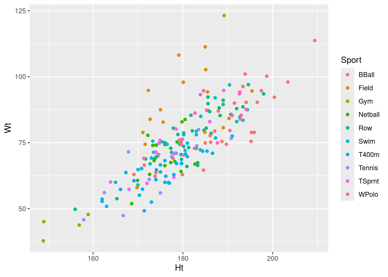

The reason for giving you the axes to use is (i) neither variable is really a response, so it doesn’t actually matter which one goes on which axis, and (ii) I wanted to give the grader something consistent to look at.

\(\blacksquare\)

Explain briefly why a multinomial model (multinom from nnet) would be the best thing to use to predict sport played from the other variables.

Solution

The categories of Sport are not in any kind of order, and there are more than two of them. That’s really all you needed, for which two marks was kind of generous.

\(\blacksquare\)

Fit a suitable model for predicting sport played from height and weight. (You don’t need to look at the results.) 100 steps isn’t quite enough, so set maxit equal to a larger number to allow the estimation to finish.

Solution

120 steps is actually enough, but any number larger than 110 is fine. It doesn’t matter if your guess is way too high. Like this:

library(nnet)
sport.1 <- multinom(Sport ~ Ht + Wt, data = athletes, maxit = 200)

# weights:  40 (27 variable)
initial  value 465.122189 
iter  10 value 410.089598
iter  20 value 391.426721
iter  30 value 365.829150
iter  40 value 355.326457
iter  50 value 351.255395
iter  60 value 350.876479
iter  70 value 350.729699
iter  80 value 350.532323
iter  90 value 350.480130
iter 100 value 350.349271
iter 110 value 350.312029
final  value 350.311949 
converged

As long as you see the word converged at the end, you’re good.

\(\blacksquare\)

Demonstrate using anova that Wt should not be removed from this model.

Solution

The idea is to fit a model without Wt, and then show that it fits significantly worse. This converges in less than 100 iterations, so you can have maxit or not as you prefer:

sport.2 <- update(sport.1, . ~ . - Wt)

# weights:  30 (18 variable)
initial  value 465.122189 
iter  10 value 447.375728
iter  20 value 413.597441
iter  30 value 396.685596
iter  40 value 394.121380
iter  50 value 394.116993
iter  60 value 394.116434
final  value 394.116429 
converged

anova(sport.2, sport.1, test = "Chisq")

The P-value is very small indeed, so the bigger model sport.1 is definitely better (or the smaller model sport.2 is significantly worse, however you want to say it). So taking Wt out is definitely a mistake.

This is what I would have guessed (I actually wrote the question in anticipation of this being the answer) because weight certainly seems to help in distinguishing the sports. For example, the field athletes seem to be heavy for their height compared to the other athletes (look back at the graph you made).

drop1, the obvious thing, doesn’t work here:

drop1(sport.1, test = "Chisq", trace = T)

trying - Ht

Error in if (trace) {: argument is not interpretable as logical

I gotta figure out what that error is. Does step?

step(sport.1)

Start:  AIC=754.62
Sport ~ Ht + Wt

trying - Ht 
# weights:  30 (18 variable)
initial  value 465.122189 
iter  10 value 441.367394
iter  20 value 381.021649
iter  30 value 380.326030
final  value 380.305003 
converged
trying - Wt 
# weights:  30 (18 variable)
initial  value 465.122189 
iter  10 value 447.375728
iter  20 value 413.597441
iter  30 value 396.685596
iter  40 value 394.121380
iter  50 value 394.116993
iter  60 value 394.116434
final  value 394.116429 
converged
       Df      AIC
<none> 27 754.6239
- Ht   18 796.6100
- Wt   18 824.2329

Call:
multinom(formula = Sport ~ Ht + Wt, data = athletes, maxit = 200)

Coefficients:
        (Intercept)         Ht          Wt
Field      59.98535 -0.4671650  0.31466413
Gym       112.49889 -0.5027056 -0.57087657
Netball    47.70209 -0.2947852  0.07992763
Row        35.90829 -0.2517942  0.14164007
Swim       36.82832 -0.2444077  0.10544986
T400m      32.73554 -0.1482589 -0.07830622
Tennis     41.92855 -0.2278949 -0.01979877
TSprnt     51.43723 -0.3359534  0.12378285
WPolo      23.35291 -0.2089807  0.18819526

Residual Deviance: 700.6239 
AIC: 754.6239

Curiously enough, it does. The final model is the same as the initial one, telling us that neither variable should be removed.

\(\blacksquare\)

Make a data frame consisting of all combinations of Ht 160, 180 and 200 (cm), and Wt 50, 75, and 100 (kg), and use it to obtain predicted probabilities of athletes of those heights and weights playing each of the sports. Display the results. You might have to display them smaller, or reduce the number of decimal places¹⁴ to fit them on the page.

Solution

To get all combinations of those heights and weights, use datagrid:

new <- datagrid(model = sport.1, Ht = c(160, 180, 200), Wt = c(50, 75, 100))
new

(check: \(3 \times 3 = 9\) rows.)

Then predict:

p <- cbind(predictions(sport.1, newdata = new))
p

I saved these, because I want to talk about what to do next. The normal procedure is to say that there is a prediction for each group (sport), so we want to grab only the columns we need and pivot wider. But, this time there are 10 sports (see how there are \(9 \times 10 = 90\) rows, with a predicted probability for each height-weight combo for each sport). I suggested reducing the number of decimal places in the predictions; the time to do that is now, while they are all in one column (rather than trying to round a bunch of columns all at once, which is doable but more work). Hence:

p %>% 
  mutate(estimate = round(estimate, 2)) %>% 
  select(group, estimate, Ht, Wt) %>% 
  pivot_wider(names_from = group, values_from = estimate)

This works (although even then it might not all fit onto the page and you’ll have to scroll left and right to see everything).

If you forget to round until the end, you’ll have to do something like this:

p %>% 
  select(group, estimate, Ht, Wt) %>% 
  pivot_wider(names_from = group, values_from = estimate) %>% 
  mutate(across(BBall:WPolo, \(x) round(x, 2)))

In words, “for each column from BBall through WPolo, replace it by itself rounded to 2 decimals”.

There’s nothing magic about two decimals; three or maybe even four would be fine. A small enough number that you can see most or all of the columns at once, and easily compare the numbers for size (which is hard when some of them are in scientific notation).

Extra: you can even abbreviate the sport names, like this:

p %>% 
  mutate(estimate = round(estimate, 2),
         group = abbreviate(group, 3)) %>% 
  select(group, estimate, Ht, Wt) %>% 
  pivot_wider(names_from = group, values_from = estimate)

Once again, the time to do this is while everything is long, so that you only have one column to work with.¹⁵ Again, you can do this at the end, but it’s more work, because you are now renaming columns:

p %>% 
  mutate(estimate = round(estimate, 2)) %>% 
  select(group, estimate, Ht, Wt) %>% 
  pivot_wider(names_from = group, values_from = estimate) %>% 
  rename_with(\(x) abbreviate(x, 3), everything())

rename doesn’t work with across (you will get an error if you try it), so you need to use rename_with¹⁶. This has syntax “how to rename” first (here, with an abbreviated version of itself), and “what to rename” second (here, everything, or BBall through WPolo if you prefer).

\(\blacksquare\)

For an athlete who is 180 cm tall and weighs 100 kg, what sport would you guess they play? How sure are you that you are right? Explain briefly.

Solution

Find this height and weight in your predictions (it’s row 6). Look along the line for the highest probability, which is 0.85 for Field (that is, field athletics). All the other probabilities are much smaller (the biggest of the others is 0.06). So this means we would guess the athlete to be a field athlete, and because the predicted probability is so big, we are very likely to be right. This kind of thought process is characteristic of discriminant analysis, which we’ll see more of later in the course. Compare that with the scatterplot you drew earlier: the field athletes do seem to be distinct from the rest in terms of height-weight combination. Some of the other height-weight combinations are almost equally obvious: for example, very tall people who are not very heavy are likely to play basketball. 400m runners are likely to be of moderate height but light weight. Some of the other sports, or height-weight combinations, are difficult to judge. Consider also that we have mixed up males and females in this data set. We might gain some clarity by including Sex in the model, and also in the predictions. But I wanted to keep this question relatively simple for you, and I wanted to stop from getting unreasonably long. (You can decide whether you think it’s already too long.)

\(\blacksquare\)

For this, use round.↩︎
If you do not take out the NA values, they are shown separately on the end of the summary for that column.↩︎
The American Green party is more libertarian than Green parties elsewhere.↩︎
Northern Ireland’s political parties distinguish themselves by politics and religion. Northern Ireland has always had political tensions between its Protestants and its Catholics.↩︎
There are three political parties; using the first as a baseline, there are therefore \(3-1=2\) coefficients for each variable.↩︎
It amuses me that Toronto’s current (2021) mayor, named Tory, is politically a Tory.↩︎
When you have variables that are categories, you might have more than one individual with exactly the same categories; on the other hand, if they had measured Size as, say, length in centimetres, it would have been very unlikely to get two alligators of exactly the same size.↩︎
Discovered by me two minutes ago.↩︎
The first render after you put this in, it will have to run it again, so you won’t save any time there: it has to create a saved version to use in the future. But the second time, if you haven’t changed this code chunk, you will definitely see a speedup.↩︎
I know I just said not to do this kind of thing, but counting is really fast, while unnecessary predictions are really slow.↩︎
There is only one district, so we can just put that in here.↩︎
The same thing applies if you are doing something like webscraping, that is to say downloading stuff from the web that you then want to do something with. Download it once and save it, then you can take as long as you need to decide what you’re doing with it.↩︎
Statistical significance as an idea grew up in the days before “big data”.↩︎
For this, use round.↩︎
abbreviate comes from base R; it returns an abbreviated version of its (text) input, with a minimum length as its second input. If two abbreviations come out the same, it makes them longer until they are different. It has some heuristics to get things short enough: remove vowels, then remove letters on the end.↩︎
Which I learned about today.↩︎